[Last Updated: 2020.02.23]
This note summarises the online course, Probabilistic Graphical Models Specialization on Coursera.
Any comments and suggestions are most welcome!
Table of Contents
- Representations
- Bayesian Network (directed graph)
- Markov Network (undirected graph)
- Inference
- Conditional Probability Queries (Overview)
- MAP (Maximum A Posterior) Inference (Overview)
- Variable Elimination (Computing Conditional Probabilities, Exact Inference)
- Belief Propagation Algorithms (Computing Conditional Probabilities, Exact Inference)
- MAP Algorithms (Finding The Most Likely Assignment)
- Sampling Methods (Using Random Sampling to Provide Approximate Conditional Probability)
- Inference in Temporal Models
- Summary
- Learning
- Summary
Representations
Bayesian Network (directed graph)
Defination
A directed acyclic graph (DAG) whose nodes represents the random variables, $X_1$, $X_2$, … $X_n$; For each node, $X_i$, we have a conditional probability distribution (CPD): $p(x_i|Par_G(Xi))$.
$Par_{G(Xi)}$ is the parents of $X_i$.
The bayesian network represents a joint distribution via the chain rule:
$p(X_1, X_2, …, X_n) = \prod_i p(X_i | Par_G(X_i))$
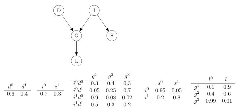
Example: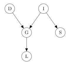
$p(D,I,G,S,L)=p(D)P(I)P(G|I,D)P(S|I)P(L|G)$
It is a legal distribution: $p \ge 0$ and $\sum_{D,I,G,S,L}p(D,I,G,S,L)=1$
Reasoning Patterns in Bayesian Network
Causal Reasoning (top to bottom)
$p(l^1) \approx 0.5$, the probability of getting the reference letter(l=1) for a student when we don’t know any information about him, is 0.5.
$p(l^1 \mid i^0) \approx 0.39$, if we know the student’s intelligence is not excellent (i=0), the probablility of getting the reference letter (l=1) is lower than that of when we don’t know his intelligence level.
Evidence Reasoning (bottom to top)
Given the student’s grade of a course, that is grade C (g=3) which is not a good performance, we can infer the probability of, the course is a difficult one (d=1) and the student has high-level intelligence (i=1) as follows:
$p(d^1\mid g^3) \approx 0.63$
$p(i^1\mid g^3) \approx 0.08$
Intercausal Reasoning (intercausal reasoning between causes)
$p(i^1 \mid g^3, d^1) \approx 0.11$, given the student get grade C and the course is hard. Here is another example which is also the example for the case of “explaining away“:
$p(i^1) \approx 0.3$, if we don’t know any information about the student;
$p(i^1 \mid g^2) \approx 0.175$, given the student got grade B;
$p(i^1 \mid g^2,d^1) \approx 0.34$, given the student got grade B for this course and the course is hard.
We can see that: the variables D and I become conditionally dependent given their commen child G is observed, even if they are marginally independent, i.e. $p(D,I)=p(D)p(I)$ (when the commen child G is not observed).
Longer Path of Graph
We can also have longer reasoning on a graph:
Example1
$p(d^1)=0.4$
$p(d^1 \mid g^3) \approx 0.63$
$p(d^1 \mid g^3,s^1)\approx0.76$, $s^1$ is the student got a high SAT score.
Exmaple2
$p(i^1)=0.3$
$p(i^1\mid g^3)\approx0.08$
$p(i^1\mid g^3,s^1)\approx0.58$
Flow of Probabilistic Influence (Active Trial)
When can X influence Y (condition on X can change the beliefs\probablities of Y)?
X CAN influence Y:
$X\rightarrow Y$,
$X\leftarrow Y$
$X\rightarrow W \rightarrow Y$
$X\leftarrow W \leftarrow Y$
$X\leftarrow W \rightarrow Y$
X CANNOT influence Y:
$X\rightarrow W \leftarrow Y$ (V Structure)
Active Trails
A trial $X_1-X_2-…-X_n$ is active if it has no V-structures ($X_{i-1}\rightarrow X_i \leftarrow X_{i+1}$).
When can X infludence Y given evidence about Z which is observed?
X CAN influence Y:
$X\rightarrow Y$
$X\leftarrow Y$
$X\rightarrow W \rightarrow Y$ ($W\not\in Z$, i.e. $W$ is not observed)
$X\leftarrow W \leftarrow Y$ ($W\not\in Z$, i.e. $W$ is not observed)
$X\leftarrow W \rightarrow Y$ ($W\not\in Z$, i.e. $W$ is not observed)
$X\rightarrow W \leftarrow Y$ ($W\in Z$, i.e. $W$ is observed), either if $W$ or one of its descendants is in $Z$.
X CANNOT influence Y:
$X\rightarrow W \rightarrow Y$ ($W\in Z$, i.e. $W$ is observed)
$X\leftarrow W \leftarrow Y$ ($W\in Z$, i.e. $W$ is observed)
$X\leftarrow W \rightarrow Y$ ($W\in Z$, i.e. $W$ is observed)
$X\rightarrow W \leftarrow Y$ ($W\not\in Z$, i.e. $W$ is not observed), if $W$ and all its descendants are not observed.
Active Trails
A trial $X_1-X_2-…-X_n$ is active given $Z$ if:
- for any V-structure ($X_{i-1}\rightarrow X_i \leftarrow X_{i+1}$), we have that $X_i$ or one of its descendants $\in Z$
- no other $X_i$ is in $Z$ (i.e. $X_i$ is not in V-structure).
Back to Table of Contents
Independencies
- For events $\alpha$ and $\beta$, $p \models \alpha \perp \beta$ ($\models$: satisfied; $\perp$: independent) if:
- $p(\alpha, \beta)=p(\alpha)p(\beta)$
- $p(\alpha \mid \beta)=p(\alpha)$
- $p(\beta \mid \alpha)=p(\beta)$
- For random variables X and Y, $p \models X\perp Y$ if:
- $p(X, Y)=p(X)p(Y)$
- $p(X \mid Y)=p(X)$
- $p(Y \mid X)=p(Y)$
Conditional Independencies
- For random variables X, Y, Z, $p \models (X \perp Y \mid Z)$ ($P(X,Y,Z)\propto \phi_1(X,Z)\phi_2(Y,Z)$) if:
- $p(X, Y \mid Z)=p(X\mid Z)p(Y\mid Z)$
- $p(X \mid Y, Z)=p(X\mid Z)$
- $p(Y \mid X, Z)=p(Y\mid Z)$
Example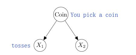
$p \nvDash X_1 \perp X_2$
But, $p \models (X_1 \perp X_2 \mid Coin)$
(Also, conditionaing can also lose independences)
d-seperation
Definiation: X and Y are d-seperated in a directed graph G given Z if there is no active trial in G between X and Y given Z.
Notation: $d$-$sep_G(X,Y\mid Z)$
Any node is d-seperated from its non-descendants given its partens, $p(X_1,X_2,…,X_n)=\prod_i p(X_i\mid Par_G(X_i))$
I-Maps (Indenpendency Map)
d-seperation in G $\Rightarrow$ P, a distribution, satisfies corresponding independence statement
$I(G)={(X\perp Y \mid Z):d\text{-}sep_G(X,Y|Z)}$ (all the independences)
Definiation: if P satisfied I(G), we say that G is an I-map (Independency map) of P
Back to Table of Contents
Factorisation and I-Maps
Theorem:
- if P factorises over G, then G is an I-map for P
- if G is an I-map for P, then P factorises over G
2 equivalent views of graph structure:
- Factorisation: G allows P to be represented
- I-map: Independencies encoded by G hold in P
Naive Bayes
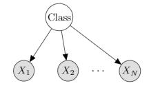
$X_1 \dots X_N$: observation (features)
($X_i \perp X_j \mid C$) for all $X_i, X_j$
$P(C, X_1, X_2, …, X_N)$ = $p(C)\prod_{i=1}^Np(X_i\mid C)$
$\frac{p(C=c1\mid X_1, X_2, \dots, X_N)}{p(C=c2\mid X_1, X_2, \dots, X_N)}=\frac{p(C=c1)}{p(C=c2)}\prod_{i=1}^N\frac{p(X_i\mid C=c1)}{p(X_i\mid C=c2)}$
Example: Bernoulli Naive Bayes for Text Classification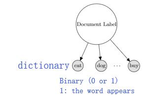
Example: MultinomialNaive Bayes for Text Classification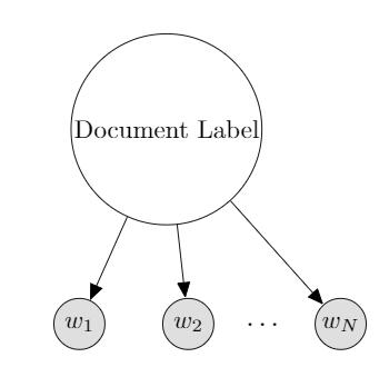
$N$: the length of this document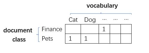
In order to obtain the probabilities, firstly, calculate the word frequency in each document category based on the dataset; Secondly, normalise each row therefore each element in this big table would be valid probability.
- This model was surprisingly effective in domains with many weakly relevant features.
- Strong independence assumptions reduce performance when many features are strongly correlated.
Back to Table of ContentsTemplate Models
Temporal Models (involve over time)
Markov Assumption
$p(X^{0:T})=p(X^0)\prod_{t=0}^{T-1}p(x^{t-1}\mid x^{0:t})$
The assumption is that: ($X^{t+1} \perp X^{0:t-1} \mid X^t$)
Therefore, the joint distribution over the entire sequence will be:
$p(X^{0:T})=p(X^0)\prod_{t=0}^{T-1}p(x^{t-1}\mid x^{t})$
Example: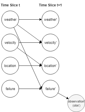
$p(w’,v’,l’,f’,o’|w,v,l,f)=p(w’|w)p(v’|w,v)p(l’|l,v)p(f’|f,w)p(o’|l’,f’)$
Initial state distribution: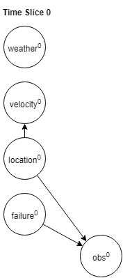
$p(w^0,v^0,l^0,f^0,o^0)=p(w^0)p(v^0|l^0)p(l^0)p(f^0)p(o^0|l^0,f^0)$
2 Time-Slice Bayesian Network (2TBN)
A Template variable $X(u_1,u_2,…,u_k)$ is instantiated duplicated multiple times and share parameters (conditional probability distribution, CPD).
Example:
Difficulty(course), Intelligence(Student), Grade(Course, Student)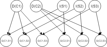
A transioin model (2TBN) over template variables $X_1,X_2,…,X_N$ is specified as a Bayesian network fragment such that:
- the nodes include $X_1’,…,X_N’$ at time t+1 and a subset of $X_1,…,X_N$ (the time t variables directly affect the state of t+1)
- only the nodes $X_1’,…,X_N’$ have parents and CPD, conditional probability distribution.
Example:
Back to Table of ContentsPlate Models
Parameter Sharing
Nested Plates
Overlapping Plates
Conditional Probability Distribution (CPD)
General CPD
- CPD $p(X|Y_1,Y_2,…,Y_K)$ specifies distribution over X for each assignment $y_1,y_2,…,y_k$
- can use any function to specify a factor $\phi(x,y_1,y_2,…,y_k)$ such that $\sum_X\phi(X,Y_1,…,Y_K)=1$ for all $y_1,…,y_k$
Table-based CPD
A table-based representation of a CPD in a Bayesian network has a size that grows exponentially in the number of parents. There are a variety of other form of CPD that explorit some type of structure in the dependency model to allow for a much more compact representation.
Back to Table of Contents
Context-specific Independence
$p \models (X \perp_c Y | Z, c)$, X a set of variables and c a particular assignment.
$p(X,Y|Z,c) = p(X|Z,c)p(Y|Z,c)$
$p(X|Y,Z,c)=p(X|Z,c)$
$p(Y|X,Z,c)=p(Y|Z,c)$
Tree-Structured CPD

Multiplexer CPD

Noise OR CPD
Y is true if someone succeed in making it true.
Sigmoid CPD

Continuous Variables

Linear Gaussian
Conditional Linear Gaussian
Non-Linear Gaussians
Back to Table of Contents
Markov Network (undirected graph)
Markov Network Fundamentals
Pairwise Markov Networks

A Pairwise Markov Network is an undirected graph whose nodes are $x_1,…,x_u$.
Each edge $x_i - x_j$ is associated with a factor (potential):
$\phi_{ij}(i,j)$
General Gibbs Distribution (a more general expression)
Even for a fully connected pairwise markov network, it is not fully expressive (i.e., it can not represent any probability distribution over random variables, not sufficiently expressive to capture all probability distribution).
Example:
For the above fully connected pairwise Markov network, we will have $C_4^2 edges * 2^2$ assignments, $O(n^2d^2)$. n is the number of edges and d is the number of how many possible values each variable can take on. However, for a general markov network, the complexity of assignments is $O(d^n)$ which is much larger than $O(n^2d^2)$. Therefore, we need a general representation method to increase the coverage.
Gibbs Distribution (represents distribution as a product of factors)
Induced Markov Network (connects every pair of nodes that are in the same factor)
Example:
More general:
Induced Markov Network $H_{\phi}$ has an edge $X_i-X_j$ whenever there exists $\phi_m \in \phi, s.t., X_i, X_j \in D_m$
Back to Table of Contents
Factorization
P, a probability distribution, factorised over H (the induced graph for $\phi$) if:
there exists $\phi={\phi_i(D_i)}={\phi_1(D_1),\phi_2(D_2),…,\phi_k(D_k)}$
such that:
$p=p_{\phi}$ (normalised product of factors)
Active Trials in Markov Network: A trial $X_1-…-X_N$ is active given $Z$ (observed) if no $X_i$ is in Z.
Conditional Random Fields
Not to model p(X,Y) but trying to model p(Y|X). X is the input and Y is the target variable.
CRF representation
CRF and Logistic Model (an example of CRF representation)
CRF for languages
The features could be:
is word capitalised, word in atlas or name list, the previous word is “Mrs”, the next word is “Times” etc.
the goal of CRF for languages is p(labels|words)
Summary for CRF
- A CRF is parameterised the same as a Gibbs distribution, but normalised differently p(Y|X)
- The CRF model do not need to model distribution over variables, we only care the prediction
- allows models with highly expressive features, without worrying about wrong independencies

Independencies in Markov Networks
Definition:
X and Y are seperated in H (Induced Markov Network Graph) given Z, if there is no active trial in H between X and Y given Z (i.e., no node along trial in Z)
Example:
Theorem:
if a probability distribution P factorised over H, and $sep_H$(X,Y|Z)
then P satisfied $(X\perp Y|Z)$
For the set which includes independencies, $I(H)={(X\perp Y|Z):sep_{H}(X,Y|Z)}$, if P satisfies I(H), we say that H is a I-map (independency map) of P
Theorem: if P factorises over H, the H is an I-Map of P
Theorem (Independence => factorisation):
For a positive distribution P (p(x)>0), if H is an I-map of P, the P factorises over H.
We can summarise that:
- Factorisation: H allows P to be represented.
- I-map: Independencies encoded by H hold in P
I-maps and perfect maps
Perfet maps capture independencies in a distribution P, $I(P)={(X\perp Y|Z): P \models (X\perp Y|Z)}$.
P factorises over G => G is an I-map for P, $I(G)\subseteq I(P)$
However, not always vice versa, there can be independencies in I(P) that are not in I(G).
If the graph encodes more independencies,
- it is sparser (has few parameters. We want a sparse graph actually)
- and more informative (we want a graph that captures as much of the structure in P as possible)
Minimal I-map
A minimal I-map does not have redundant edges.
A minimal I-map may still cannot capture I(P). A minimal I-map may fail to capture a lot of structure even if they are presented in the distribution and even if it is representable as a Bayes net or as a graphical model.
Example:
if remove the red edge, $D\perp G$; if remove the green one, $I\perp G|D$; if remove the purple one, $D\perp I | G$. They are not the case in our original distribution. None of them can be removed. Therefore, this is also a minimal I-map.
A perfect map $I(G)=I(P)$, means G perfectly captures independencies in P. Unfortunately, a perfect map are hard to come by.
Example of doesn’t have a perfect map:
IF we consider using Bayes net as perfect maps:
Another imperfect map:
IF we consider Markov network as a perfect map:
Perfect map: $I(H)=I(P)$, (here we use a different symbol replace G by H), H perfectly captures independencies in P (a perfect map is great, but may not exist)
Converting BNs <—> MNs losses independencies:
- BN to MN: loss independencies in V-structure
- MN to BN: must add triangulating edges to loops
Uniqueness of perfect map
Formal Definition: I-equivalence
Two graphs G1 and G2 over X1 … Xn are I-equivalent if I(G1)=I(G2) (examples above)
Most Gs have many I-equivalent variants.
I-equivalence is an important notion. It tells us: there are certain aspects of the graphical model are unidentifiable, which means that if we end up for whatever reason thinking this is the graph that represent our probability distribution, it could just as easyly as this one or that one. So without prior knowledge of some kind or another, for example that we prefer X to be a parent of Y, there is no way for us to select among these different choices.
Local Structure in Markov Networks
Log-linear Models (CRF, Ising Model, Metric MRFs)
The local structure means we do not need full table representations in both directed and undirected models. Here we will discuss the local structure in undirected models.

- each feature $f_j$ has a score $D_j$
- different featrues can have same scope
Example 1:
Example 2 (CRF):
Example 3 (Ising Model, pair-wise Merkov Network, Joint Spins):
Example 4 (Metric MRFs):
All $X_i$ take values in label space V
Distance function $\mu: V*V\to R^{+}$ (non-negative)
We have a feature:
we want lower distantce (higher probability).
lower probability, if the values of Xi and Xj far in $\mu$.
Examples of $\mu$:

$\mu(v_k,v_l)=min(|v_k-v_l|,d)$
Shared features in Log-Linear Models
In most MRFs, same features and weights can be used over many scopes.
- Ising Model

Here, $X_iX_j$ is the feature function, $f(X_i,X_j)$. - CRF

1) same energy terms $w_k f_k(x_i,y_i)$ repeat for all positions i in the sequence.
2) same energy terms $w_m f_m(y_i,y_{i+1})$ repeat for all positions i
Summary:
Repeated Features:
1) need to specify for each feature $f_k$ a set of scopes, Scopes[$f_k$]
2) for each $D_k \in Scope[f_k]$ we have a term $w_kf_k(D_k)$ in the energy function: $w_k\sum f_k(D_k), D_k \in Scopes(f_k)$. Example: Scope[$f_k$] = {Yi,Yj; i and j are adjacient}
Decision Making
Maximum Expected Utility
Simple Decision Making:
A simple dicision making situation D:
- A set of possible actions Val(A)={$a^1,…,a^k$}, different choices
- A set of states Val(X)={$x_1,…,x_N$}, states of the world
- A distribution p(X|A)
- A utlity function U(X,A)
The expected utility:
D is the situation and a is the one of the actions.
We want to choose action a that maximise EU:
$a^*=\text{argmax}_a EU[D(a)]$
Simple Influence Diagram
- Note that: Action is not a random variable, so it does not have a CPD (conditional probability distribution)

EU[$f_0$]=0
*EU[$f_1$]=0.5(-7)+0.35+0.2*20=2
More complex Influence Diagram
$V_G, V_S$ and $V_Q$ represent different components of the utility function (a decomposed utility).
$V=V_G + V_S + V_Q$
Information Edges
The survey here means that conducting a survey to investigate the market demand.
Expected utility with Information:
EU[D[$\delta_A$]]=$\sum_{x,a}P_{\delta_A}(X,a)U(X,a)$, a joint probability distribution over X $\cup$ {A}.
Decision rule $\delta$ at action node A is a CPD, P(A|parents(A)), here is P(F|S). $\delta_A$ is a decision rule for an action.
We want to choose the decision rule $\delta_A$ that maximises the expected utility $argmax_{\delta_A}EU[D[\delta_A]]$. (MEU(D)=$\max_{\delta_{A}}EU[D[\delta_{A}]]$).
Example:
To maximise the summination: the optimal decision rule is:
0+1.15+2.1=3.25 (the agent overall expected utility in this case)
More generally
A: actions
Summary
- treat A as a random variable with arbitrary (unknown) CPD, $\delta_A(A|Z)$
- introduce utility factor with scope $P_{a_U}$, P is parent, u is utility
- eliminate all variables except A, Z (A’s parents) to produce factor $\mu(A,Z)$
- for each Z (observation) set: we choose the optimal decision rule:
Utility Functions
Lotteries Example:
we can use expected utility to decide which to buy between 2 different lotteries.
1) 0.2U($4) + 0.8U($0)
2) 0.25U($3) + 0.75U($0)
Utility Curve

Multi-Attribute Utilities
- All attributes affecting preferences (e.g., money, time, pleasure, …) must be integrated into one utility function;
- Example: Micromorts 1/1000000 chance of death worth ($\approx $$20, 1980); QALY (quality-adjusted life year)
Example (prenatal diagnosis):
Break down the utility function as a sum of utilities, $U_1(T) + U_2(K) + U_3(D,L) + U_4(L,F)$
Value of Perfect Information
(Another question: which observations should I even make before making a decision? Which one is worthwhile and which one is not?)
- VPI(A|X) is the value of observing X before choosing an action at A
- $D$: original influence diagram
- $D_{x\to A}$: influence diagram with edge $x \to A$
, MEU is maximum expected utility
Example:
First find the MEU decision rules for both and then compute $MEU(D_{x\to A})-MEU(D)$.
As shown below: $MEU(D_{x\to A})-MEU(D)=3.25-2=1.25$, which means the agent should be willing to pay anthing up to 1.25 utility points in order to conduct the survey.
Theorem
$VPI(A|X) := MEU(D_{x\to A})-MEU(D), VPI(A|X) >= 0$
$VPI(A|X)=0$, if and only if the optimal decision rule for D is still optimal for $D_{x\to A}$.
Detailed Example:
If the agent does not get any information (observation):
$EU(D[C_1])=0.1\times0.1+0.2\times0.4+0.7\times0.9=0.72$
$EU(D[C_2])=0.04+0.2+0.09=0.33$
What if the agent get to make an observation?
The expected utility (EU) (with observation) is:
- if the agent choose company2, and its state is poor ($S_2=poor$), the EU is 0.1 (stick the original idea, which prefers company1, because the EU is lowere than 0.72)
- if the agent choose company2, and its state is moderate, the EU is 0.4 (stick the original idea, which prefers company1, because the EU is lowere than 0.72)
- if the agent choose company2, and its state is great, the EU is 0.9 (prefer company2, change mind to company2)
Therefore, the optimal decision rule is:
$\delta_A(C|S_2)= P(C^2)=1, if S_2=S^3 (great)$
$\delta_A(C|S_2)= P(C^1)=1, otherwise$
In this scenario, the MEU value is 0.743.
$MEU(D_{S_2\to C})=\sum_{S_2,C}\delta(C|S_2)\mu(S_2,C)=0.743$
0.743 is not a significant improvement over our original MEU value. If observing, the agent shouldn’t be willing to pay his company too much money in order to get information about the detail.
Another situation (neither company doing great):
$EU(D[C_1])=0.35$
$EU(D[C_2])=0.04+0.2+0.09=0.33$
$\delta_A(C|S_2)= P(C^2)=1, if S_2=S^2, S^3 (great)$
$\delta_A(C|S_2)= P(C^1)=1, otherwise$
$MEU(D_{S_2\to C})=\sum_{S_2,C}\delta(C|S_2)\mu(S_2,C)=0.43$
0.43 is much more significant increase.
Third situation (neither company doing great):
$EU(D[C_1])=0.788$
$EU(D[C_2])=0.779$
$\delta_A(C|S_2)= P(C^2)=1, if S_2=S^2, S^3 (great)$
$\delta_A(C|S_2)= P(C^1)=1, otherwise$
$MEU(D_{S_2\to C})=\sum_{S_2,C}\delta(C|S_2)\mu(S_2,C)=0.8142$
In this situation, in the bubble days of the Internet boom and pretty much companys gets funded, with a pretty high probability even if their business models are dubious.
(only a small fairly small increase over 0.788 that they could have already guaranteed themselves without making that observation)
Knowledge Engineering
Generative vs. Discriminative
- Generative: when don’t have a preditermined task (task shifts). Example: medical diagnosis pack: every patient present differently, each patient case, we have different subset of things happend to know (symptoms and tests), we want to measure some variables and predict others; easy to train in certain regimes. (where data is not fully labelled)
- Discriminative: particalar prediction task, need richly expressive features (avoid dealing with corelations), and can achive high performance.
Designing a graphical model (variable types)
- Target: there are the ones we care about, e.g., a set of diseases in the diagnosis setting
- Observed: not necessary care predicting them, like symptoms and test results in the medical setting
- Latent/hidden: which can simply our structure, example below:

Structure
- Causal versus non-causal ordering.
Do the arrows in directed graph corresponding to causality? (Yes and No)
No: $X\to Y$ any distribution that we can model on this graphical model where X is a parent of Y, we can equally well model in a model $Y\to X$. In some examples, we can reverse edges and have a model that’s equally expressive. (But the model might be nasty, examples below. Thus the causal ordring is generally more sparser, intuitive and more easier to parameterise)
Parameters: Local Structure
| Context-Specific | Aggregating | |
|---|---|---|
| Discrete | tree-CPDs | sigmoid CPDs |
| Continuous | regression tree (continues version of tree CPD, breaks up the context based on some thresholds on the continuous variables) | Linear Gaussian |
Iterative Refinement
- Model testing (ask queries and see whether the answers coming out are reasonable)
- sensitivity analysis for parameter: look at a given query, and ask which parameters have the biggest different on the value of the query, and that means those are probably the ones we should fine tune in order to get best results)
- Error Analysis
- add features
- add dependencies
Inference
Overview: how to use the these declarative representation to answer actual queries.
Conditional Probability Queries (Overview)
Evidence: E = e, set of observations
Query: a subset of variables Y
Task: compute p(Y|E=e) (NP-Hardness)
Sum-Product in Bayes Network and Markov Network
Given a PGM $P_{\phi}$ (defined by a set of variables X and factors), value $x \in Val(X)$, and we need compute $P_{\phi}(X=x)$
Example:
Note that each of the CPDs converts a factor over the scope of the family (e.g., P(G|I,D)->$\phi_G(G,I,D)$).
If we need to know P(J), we need to compute the follows:
For the sum-product in MN:
Evidence: Reduced Factors
$p(Y|E=e)=\frac{P(Y,E=e)}{P(E=e)}$
Define: W = {$X_1,X_2,…,X_n$} - Y - E
Example:
If we want to compute p(J|I=i, H=h), we can just compute the above equation and re-normalise.
Summary of Sum-Product Algorithm
$p(Y|E=e)=\frac{P(Y,E=e)}{P(E=e)}$, Y is the query.
numerator: $p(Y,E=e)=\sum_w\frac{1}{Z}\prod_k\phi_k’(D_k’)$, reduced by evidence.
denominator: $p(E=e)=\sum_Y\sum_w\frac{1}{Z}\prod_k\phi_k’(D_k’)$
In practice, we can compute $\sum_w\prod_k\phi’_k(D’_k)$ and renormalise.
There are many algorithms for computing conditional probability queries.
The algorithm list of conditional probability:
- Push summations into factor product
- Variable elimination (dynamic programming)
- Message passing over a graph
- Belief propagation (exact inference)
- Variational approximations (approximate inference)
- Random sampling instantiations (approximate inference)
- Markov Chain Mente Carlo (MCMC)
- Importance Sampling
MAP (Maximum A Posterior) Inference (Overview)
Evidence: E = e (observations)
Query: all other variables Y (Y = {$X_1, X_2,…,X_n$} - E)
Task: compute MAP = $argmax_YP(Y|E=e)$
Note that:
1) there may be more than one possible solution
2) MAP $\neq$ Max over margins. Example below:
The CPDs are:
P(A=0)=0.4
P(A=1)=0.6
P(B=0|A=0)=0.1
P(B=1|A=0)=0.9
P(B=0|A=1)=0.5
P(B=1|A=1)=0.5
Therefore we can get the joint distribution:
P(B=0,A=0)=0.04
P(B=1,A=0)=0.36
P(B=0,A=1)=0.3
P(B=1,A=1)=0.3
Obviously, the assignement which MAP(A,B) is A=0,B=1. Because its has the hightest probability 0.36. However, if we look at the two variables seperately, the A should be assigned as A=1 which is opposite to the A=0. Therefore, we cannot look seperately at the marginal over A and over B.
Compute MAP is a NP-Hardness problem.
Given a PGM $P_{\phi}$, find a joint assignment X with the hightest probability $P_{\phi}(X)$.
Max-Product
Example:
$p(J)=argmax_{C,D,I,G,S,L,J,H}\phi_C(C)\phi_D(C,D)\phi_I(I)\phi_G(G,I,D)\phi_S(S,I)\phi_L(L,G)\phi_J(J,L,S)\phi_H(H,D,J)$
Algorithms: MAP (there are also different algorithms to solve the problem)
- Push maximisation into factor product
- variable elimination
- Message passing over a graph
- Max-product belief propagation
- Using methods for integer programming (a general class of optimisation which is over discreet spaces)
- For some networks: graph-cut methods
- Combinatorial search (use standard search techniques over combinatorial search spaces)
Variable Elimination
The simplest and the most fundamental algorithm.
Variable Elimination Algorithm
Elimination in Chains

Ultimately, we will end up with an expression that involves only the variable E.
Elimination in a more complicated BN

Variable Elimination with Evidence

If we need to compute P(J|I=i,H=h), we just renormalise the above results.
Variable Elimination in MNs

Summary Variable Elimination Algorithm

- reduce all factors by evidence
- get a set of factors $\Phi$
- For each non-query variable Z
- Eliminate variable Z from $\Phi$
- multiply all remaining factors
- renormalising to get distribution
Complexity of Variable Elimination

Factor Product:
Factor Marginalisation:
Details:
- Start with m factors
- for Bayesian Networks, m <= n (the number of variables). m=n when one factor for each variable
- for Markov Networks, m can be larger than the number of variables
- At each elimination step generate a factor
- at most n elimination steps
- total number of factors $m^*\leqslant m+n$
- product operations: $\sum_k(m_k-1)N_k\leqslant N\sum_k(m_k-1)\leqslant Nm^*$, $N=\max(N_k)=$size of the largest factor. Each factor multiply in at most once.
- sum operations $\leqslant \sum_kN_k\leqslant N\cdot$number of elimination steps $\leqslant$ $Nn$. (Total work is linear in N and $m^*$)
$N_k=|Val(X_k)|=O(d^{rk})$ where: (exponential blow up)
- $d=\max(|Val(X_i)|)$, d values in their scope
- $r_k=|X_k|$ (number of variables in k-th factor) =cardinality of the scope of the k-th factor
Complexity of algorithm depends heavily on the elimination ordering
Graph-based Perspective on Variable Elimination
View a BN as a undirected graph:
all variables connected to I become connected directly.
Its a pretty good elimination ordering in this case.
To summarise:
Induced Graph
The induced graph $I_{\Phi,\alpha}$ over factors $\Phi$ and ordering $\alpha$:
- undirected graph
- $X_i$ and $X_j$ are connceted if they appeared in the same factor in a run of the variable elimination (eliminate factors generate new factors) algorithm using $\alpha$ as the ordering
Cliques in the Induced Graph
Theorem: Every factor produced during VE is a clique in the induced graph.
A clique is a maximal fully connected sub-graph.
Example:
(fully connected each other)
It is maximal because we cannot add any other variable to this and still have that property hold. For example, add node S, but S not connects D.
Theorem: every (maximal) clique in the induced graph is a factor produced during VE.
Induced width:
- the width of an induced graph is the number of nodes in the largest clique in the graph minus 1.
- minimal induced width of a graph K is $\min_{\alpha}$(width$(I_{k,\alpha})$), $\alpha$ over all possible elimination orders.
- it provides a lower bound on best perfromance (the best achievable complecity) of VE to a model fatorizing over K (graph K)
Finding Elimination Orderings
- Greedy seach using heuristic cost function
- at each point, eliminate node with smallest cost
- possible cost functions:
- min-neighbors: number of neighbors in current graph
- pick the node has the smallest/minimal number of neighbors
- corresponding to the smallest factor
- the one whose cardinality (the number of variables in this factor) is smallest
- min-weight: weight (e.g., number of values) of factor formed
- min-fill: number of new fill edges
- weighted min-fill: total weight of new fill edges (edge weight = product of weights of the 2 nodes)
- min-neighbors: number of neighbors in current graph
Theorem: the induced graph is triangulated.
- no loops of length $>$ 3 without a “bridge”

- can find elimination ordering by finding a low-width (little clique) triangulation of original graph $H_{\phi}$
Variable Elimination (Summary)
- Finding the optimal elimination ordering is NP-hard.
- Simple heuristics that try to keep induced graph small often provide reasonable performance.
Belief Propagation Algorithms
Message Passing in Cluster Graphs
Build a cluster graph:
Passing Messages:
Each cluster is going to send messages to its adjacent clusters that reflect the same process as above.
Cluster Graphs (Generalisation Definition)
Undirected graph
- Nodes: clusters $C_i\subseteq{X_1,…,X_n}$. $C_i$ is a subset of variables
- Edges: between $C_i$ and $C_j$ associated with subset $S_{i,j} \subseteq C_i \cap C_j$. $S_{i,j}$ is the variables that they talk about
Given a set of factors $\Phi$, assign each $\phi_k$ to a cluster $C_{\alpha(k)}$ (one and only one cluster) s.t. Scope[$\phi_k$] $\subseteq C_{\alpha(k)}$ (a subset of $C_{\alpha(k)}$)
Define $\psi_i(C_i)=\prod_{k:\alpha(k)=i}\phi_k$
- define a initial belief of a particular cluster the product of all factors that assigned to it
- and some clusters might not have have factors assigned to them, in this case equal to 1.
Example Cluster Graph
Initially we have to figure out for each of those factors a cluster in which to put it.
- For A,B,C: there is only one choice because there is only one cluster in the enitre graph that understands abouts all of A, B and C.
- For B,C: however, it has two choinces. It can go into cluster one or two. Both are fine.
- For B,D: also has two choinces.
- For D,E and B,E: they only have one choice.
- For B,D: it has 2 choices.
- For B,D,F: there is only one choice.
This is one possible way of assigning the cluster, the factor Flow of Probabilistic Influence (Active Trial)
When can X influence Y (condition on X can change the beliefs\probablities of Y)?
X CAN influence Y:
$X\rightarrow Y$,
$X\leftarrow Y$
$X\rightarrow W \rightarrow Y$
$X\leftarrow W \leftarrow Y$
$X\leftarrow W \rightarrow Y$
X CANNOT influence Y:
$X\rightarrow W \leftarrow Y$ (V Structure)
Active Trails
A trial $X_1-X_2-…-X_n$ is active if it has tno clusters.
Different Cluster Graph
For the exact same set of factors, the clusters have not changed, but the edge changes.
Message Passing
General:
Belief Propagation Algorithm
- Assign each factor $\phi_k\in\Phi$ to a cluster $C_{\alpha(k)}$
- Construct initial potentials $\Psi_i(C_i)=\prod_{k:\alpha(k)=i}\phi_k$
- Initialise all messages to be 1
- Repeat: (until When and how to select edge - different variants of algorithms will be described later on)
- select edge (i,j) and pass message. $N_i$ is the neighbour.
- select edge (i,j) and pass message. $N_i$ is the neighbour.
- Compute, belief of this cluster, $\beta_i(C_i) = \Psi_i \times \prod_{k\in N_i} \delta_{k \to i}$. $N_i$ is all the neighbors.
Belief propagation run (approximate)
Example:
The resulting beliefs are pseudo-marginals, but the algorithm actually performs well in a range of practical applications.
Properties of Cluster Graphs
Family Preservation
Given a set of factors $\Phi$, we assign each $\phi_k$ to a cluster $C_{\alpha(k)}$, s.t. Scope[$\phi_k$]$\in C_{\alpha(k)}$
For each factor $\phi_k$ in $\Phi$, there exists a cluster $C_i$ s.t. Scope[$\phi_k$] $\subseteq C_i$
Runing Itersection Property
For each pair of clusters $C_i$ and $C_j$, and variable $X\in C_i\cap C_j$, there exists a unique path between $C_i$ and $C_j$ for which all clusters and sepsets (edge) contain X.
Alternative defination of Running Itersection Property —- Equivalently: for any variable X, the set of clusters and sepsets (edges) containing X from a tree. (each variable inducing its own little tree across which information about that variable flows in the graph.)
If X and Y are very strongly correlated, BP does poorly when have sharing parameters, due to the feedback loops. The more skewed the probabilities in your graphical mode, the harder time belief propagation has in terms of the results that it gets.
Examples of Illegal Cluster Graphs:
For B, there is no way to connect the B in cluster 1 and 2 or 2 and 3. This graph violates the existence.
This vailates the uniqueness. (the loop, 2 ways between cluster 1 and 4.)
Examples of Valid Graph:
Bethe Cluster Graph (How to construct a cluster graph that has the desired properties?)
- Big Cluster: for each $\phi_k\in\Phi$, a factor cluster $C_k$ = Scope[$\phi_k$]
- Small Cluster: for each $X_i$ a singleton cluster {$X_i$} (variable)
- Edge $C_k$—-$X_i$ if $X_i\in C_k$

Summary
- Cluster graph must satisfy:
- family preservation: allow $\Phi$ to be encoded
- running intersection: connect all information about any variable, but without feedback loops
- Bethe cluster graph is often first default
- Richer cluster graph stuctures (e.g., more edges) can offer different trade-offs. wrt. computational cost (increasing the amount of sizes of the messages that are passed that can grow more expensive) but at the same time imprve the preservation of dependencies as messages are passed in the graph so that more information is actually kept and not lost in this message passing process.
Properties of Belief Propagation
Calibration
A cluster graph is calibrated if every pair of adjacent clusters $C_i$ and $C_j$ agree on their sepset $S_{i,j}$:
$\sum_{C_i-S_{ij}}\beta_i(C_i)=\sum_{C_j-S_{ij}}\beta_j(C_j)$. In other words, the marginilised beliefs are equal.
Convergence ($\to$ Calibration)
$\delta_{i\to j}(S_{ij})=\delta’_{i\to j}(S_{ij})$, equal the message at previous time step.
The expression above is corresponds to the sepset belief:
$\mu_{i,j}(S_{i,j})=\delta_{j\to i}\delta_{i\to j}=\sum_{C_j-S_{i,j}}\beta_j(C_j)$
Reparameterisation
If we write in this form:
It can be seen that it is simply the unnormalised measure. It implicates the term/ratio is simply a different set of parameters that captures the original un-normalised measure that defined our distribution.
Therefore, we have not lost information as a result of belief propagation algorithm. The distribution is still there, just a different set of parameters.
Summary
Cluster graph beliefs are an alternative, calibrated, parametorisation of the original unnormalised density.
- No information is lost by message passing.
- Reparametorised the original distribution into a more convenient and easily usable form.
Clique Trees (faster and exact answer of inference)
A speical case of cluster graph which has the performance guarantee. (faster, exact answer of inference).
Message Passing in Trees
A simple example tree:
As you can see, we have marginalised out in a legal order.
Clique Tree:
Undirected tree such that:
- nodes are clusters $C_i\subseteq{X_1…X_n}$
- edge between $C_i$ and $C_j$ associated with sepset $S_{ij}=C_i\cap C_j$
(For each pair of clusters $C_i$ and $C_j$, and variable $X\in C_i\cap C_j$, in the unique path between $C_i$ and $C_j$, all clusters and sepsets contain X)
More Complex Clique Tree:
Clique Tree Correctness:
- If X is eliminated when we pass the message $C_i \to C_j$
- Then X does not appear in the $C_j$ side of tree
Summary:
- In this case, computation is a variant of variable elimination
- Resulting beliefs are guaranteed to be correct marginals
Computation

We can compute all of the messages in this entire tree in one paths in either direction. One path is from left to right and one path from right to left. In the context of chain structures, you might see this under the name forward-backward algorithm. This is very commonly used in things like the hidden Markov model and other similar chain structured representations.
Once …