[Last Updated: 06/01/2019]
This article aims to summarise:
- basic concepts in machine learning (e.g. gradient descent, back propagation etc.)
- different algorithms and various popular models
- some practical tips and examples were learned from my own practice and some online courses such as Deep Learning AI.
If you a student who is studying machine learning, hope this article could help you to shorten your revision time and bring you useful inspiration. If you are not a student, hope this article would be helpful when you cannot recall some models or algorithms.
Moreover, you can also treat it as a “Quick Check Guide”. Please be free to use Ctrl+F to search any key words interested you.
Any comments and suggestions are most welcome!
Note
Please note that: The Wechat Public Account is available now! If you found this article is useful and would like to found more information about this series, please subscribe to the public account by your Wechat! (2020-04-03)
Table of Contents
- Activation Functions
- Gradient Descent
- Computation Graph
- Backpropagation
- Gradients for L2 Regularization (weight decay)
- Vanishing/Exploding Gradients
- Mini-Batch Gradient Descent
- Stochastic Gradient Descent
- Choosing Mini-Batch Size
- Gradient Descent with Momentum (always faster than SGD)
- Gradient Descent with RMSprop
- Adam (put Momentum and RMSprop together)
- Learning Rate Decay Methods
- Batch Normalization
- Parameters
- Regularization
- Models
- Logistic Regression
- Multi-Class Classification (Softmax Regression)
- Transfer Learning
- Multi-Task Learning
- Convolutional Neural Network (CNN)
- Filter/Kernel
- Stride
- Padding (valid and same convolutions)
- A Convolutional Layer
- 1*1 Convolution
- Pooling Layer (Max and Average Pooling)
- LeNet-5
- AlexNet
- VGG-16
- ResNet (More Advanced and Powerful)
- Inception Network
- Object Detection
- Face Verification
- Neural Style Transfer
- 1D and 3D Convolution Generalisations
- Sequence Models
- Transformer (Attention Is All You Need)
- Bidirectional Encoder Representations from Transformers (BERT)
- Practical Tips
Activation Functions
| Name | Function | Derivative |
|---|---|---|
| sigmoid | $g(z)=\frac{1}{1+e^{-z}}$ | $g(z)(1-g(z))$ |
| tanh | $tanh(z)$ | $1-(tanh(z))^2$ |
| 0, if $z<0$ | ||
| Relu | $max(0,z)$ | 1, if $z>0$ |
| undefined, if $z=0$ | ||
| 0.01, if $z<0$ | ||
| Leaky Relu | $max(0.01z,z)$ | 1, if $z>0$ |
| undefined, if $z=0$ |
Gradient Descent
Gradient Descent is an iterative method to find the local minimum of an objective function (e.g. loss function).
|
|
The symbol $:=$ means the update operation. Obviously, we are updating the value of parameter $W$.
Usually, we use $\alpha$ to represent the learning rate. It is one of the hyper parameters (we will introduce more hyper parameters in another section) when training a neural network. $J(W)$ is the loss function of our model. $\frac{dJ(W)}{dW}$ is the gradient of parameter $W$. If $W$ is a matrix of parameters(weights), $\frac{dJ(W)}{dW}$ would be a matrix of gradients of each parameter (i.e. $w_{ij}$).
Question: Why we minus the gradients not add them when minimizing the loss function?
Answer:
For example, our loss function is $J(W)=0.1(W-5)^2$ and it may look like: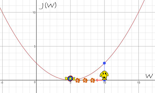
When $W=10$, the gradient $\frac{dJ(W)}{dW}=0.1*2(10-5)=1$. Obviously, if we are going to find the minimum of $J(W)$, the opposite direction of gradient (e.g. $-\frac{dJ(W)}{dW}$) is the correct direction to find the local lowest point (i.e. $J(W=5)=0$).
But sometime, gradient descent methods may suffer local optima problem.
- Computation Graph
The computation graph example was learned from the first course of Deep Learning AI.
Let’s say we have 3 learnable parameters, $a$, $b$ and $c$. The cost function is $J=3(a+bc)$. Next, we need to compute the parameters’ gradient: $\frac{dJ}{da}$, $\frac{dJ}{db}$ and $\frac{dJ}{dc}$. We also define: $u=bc$, $v=a+u$ and $J=3v$. The computation could be converted into the computation graph below: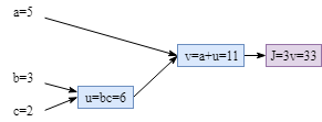
- Backpropagation
Based on the graph above, it is clear that the gradient of parameters are: $\frac{dJ}{da}=\frac{dJ}{dv}\frac{dv}{da}$, $\frac{dJ}{db}=\frac{dJ}{dv}\frac{dv}{du}\frac{du}{db}$, $\frac{dJ}{dc}=\frac{dJ}{dv}\frac{dv}{du}\frac{du}{dc}$.
Computing the gradients of each node is easy as shown below. (Tips: In fact, if you are implementing your own algorithm, the gradients could be computed during the forward process to save computation resources and training time. Therefore, when you do backpropagation, there is no need to compute the gradients of each node again.)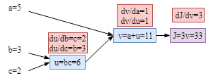
Now we can compute the gradient of each parameters by simply combine the node gradients: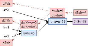
$\frac{dJ}{da}=\frac{dJ}{dv}\frac{dv}{da}=3\times1=3$
$\frac{dJ}{db}=\frac{dJ}{dv}\frac{dv}{du}\frac{du}{db}=3\times1\times2=6$
$\frac{dJ}{dc}=\frac{dJ}{dv}\frac{dv}{du}\frac{du}{dc}=3\times1\times3=9$
- Gradients for L2 Regularization (weight decay)
The gradients is changed a bit by adding $\frac{\lambda}{m}W$.
- Vanishing/Exploding Gradients
If we have a very deep neural network and we did not initialize weight properly, we may suffer gradients vanishing or exploding problems. (More details about parameter initialization: Parameters Initialization)
In order to explain what is the vanishing or exploding gradients problems, a simple but deep neural network architecture will be taken as an example. (Again, the great example is from the online course Deep Learning AI)
The neural network has $L$ layers. For simplicity, the parameter $b^{[l]}$ for each layer is 0 and all the activation functions are $g(z)=z$. In addition, every parameter $W^{[l]}$ has the same values.
Based on the simple model above, the final output would be:
$y=W^{[l]}W^{[l-1]}W^{[l-2]}…W^{[3]}W^{[2]}W^{[1]}X$
Because the weight value $1.5>1$, we will get $1.5^L$ in some elements which is explosive. Similarly, if the weight value less than 1.0 (e.g. 0.5), there are some vanishing gradients (e.g. $0.5^L$) somewhere.
These vanishing/exploding gradients will make training very hard. So carefully initializing weights for deep neural networks is important.
- Mini-Batch Gradient Descent
If we have a huge training dataset, it will take a long time that training a model on a single epoch. It would be hard for us to track the training process. In the mini-batch gradient descent, the cost and gradients are computed based on the training examples in current batch.
$X$ represents the whole train set and it is divided into several batches as shown below. $m$ is the number of training examples.

The procedure of mini-batches is as follows:
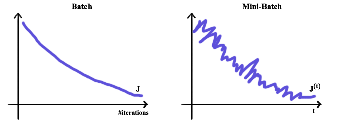
During the training process, the cost trend is smoother when we do not apply mini-batch gradient descent than that of using mini-batches to train our model.
- Stochastic Gradient Descent
When the batch size is 1, it is called Stochastic gradient descent.
- Choosing Mini-Batch Size
Mini-Batch Size:
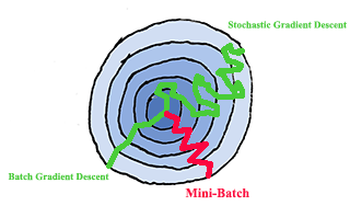
1) if the size is $M$, the number of examples in the whole train set, the gradient descent is exactly Batch Gradient Descent.
2) if the size is 1, it is called Stochastic Gradient Descent.
In practice, the size is selected somewhere between 1 and M. When $M <= 2000$, the dataset is supposed to be a small dataset, using Batch Gradient Descent is acceptable. When $M > 2000$, probably Mini-Batch Gradient Descent is a better way to train our model. Typically the mini-batch size could be 64, 128, 256, etc.
- Gradient Descent with Momentum (always faster than SGD)
On each mini-batch iteration $t$:
1) Compute $dW$, $db$ on the current mini-batch
2) $V_{dW}=\beta V_{dW}+(1-\beta)dW$
3) $V_{db}=\beta V_{db}+(1-\beta)db$
4) $W:=W-\alpha V_{dW}$
5) $b:=b-\alpha V_{db}$
The hyper parameters in momentum are $\alpha$(learning rate) and $\beta$. In momentum, $V_{dW}$ is the information of the previous gradients history. If we set $\beta=0.9$, it means we want to take the around last 10 iterations’ gradients into consideration to update parameters.
The original $\beta$ is from the parameter of exponentially weighted averages. E.g. $\beta=0.9$ means we want to take around the last 10 values to compute average. $\beta=0.999$ means considering around the last 1000 values etc.
- Gradient Descent with RMSprop
On each mini-batch iteration $t$:
1) Compute $dW$, $db$ on the current mini-batch
2) $S_{dW}=\beta S_{dW}+(1-\beta)(dW)^2$
3) $S_{db}=\beta S_{db}+(1-\beta)(db)^2$
4) $W:=W -\alpha \frac{dW}{\sqrt{S_{dW}}+\epsilon}$
5) $b:=b-\alpha \frac{db}{\sqrt{S_{db}}+\epsilon}$
- Adam (put Momentum and RMSprop together)
$V_{dW}=0$,$S_{dW}=0$,$V_{db}=0$,$S_{db}=0$
On each mini-batch iteration $t$:
1) Compute $dW$, $db$ on the current mini-batch
// Momentum
2) $V_{dW}=\beta_1 V_{dW}+(1-\beta_1)dW$
3) $V_{db}=\beta_1 V_{db}+(1-\beta_1)db$
// RMSprop
4) $S_{dW}=\beta_2 S_{dW}+(1-\beta_2)(dW)^2$
5) $S_{db}=\beta_2 S_{db}+(1-\beta_2)(db)^2$
// Bias Correction
6) $V_{dW}^{correct}=\frac{V_{dW}}{1-\beta_1^t}$
7) $V_{db}^{correct}=\frac{V_{db}}{1-\beta_1^t}$
6) $S_{dW}^{correct}=\frac{S_{dW}}{1-\beta_2^t}$
7) $S_{db}^{correct}=\frac{S_{db}}{1-\beta_2^t}$
// Update Parameters
$W:=W -\alpha \frac{V_{dW}^{correct}}{\sqrt{S_{dW}^{correct}}+\epsilon}$
$b:=b-\alpha \frac{V_{db}^{correct}}{\sqrt{S_{db}^{correct}}+\epsilon}$
The “correct” is the concept of “Bia Correction” from exponentially weighted average. The correction could make the computation of averages more accurately. $t$ is the power of $\beta$.
Usually, the default hyper parameter values are: $\beta_1=0.9$, $\beta_2=0.99$ and $\epsilon=10^{-8}$.
Learning rate $\alpha$ needs to be tune. Alternatively, applying learning rate decay methods could also work well.
- Learning Rate Decay Methods
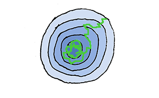
If the learning rate is fixed during train phrase, the loss/cost may fluctuate as shown in the picture below. Find way to make the learning rate adaptive could be a good idea.
Decay based on the number of epoch

Decreasing learning rate according to the number of epoch is a straightforward way. The following is the rate decay equation.
For example, the initial $\alpha=0.2$ and decay rate is 1.0. The learning rates of each epoch are:
| Epoch | $\alpha$ |
|---|---|
| 1 | 0.1 |
| 2 | 0.67 |
| 3 | 0.5 |
| 4 | 0.4 |
| 5 | … |
Of course, there are also some other learning rate decay methods.
| Other Methods | Equation |
|---|---|
| exponentially decay | $\alpha=0.95^{EpochNumber}\alpha_0$ |
| epoch number related | $\alpha=\frac{k}{EpochNumber}\alpha_0$ |
| mini-batch number related | $\alpha=\frac{k}{t}\alpha_0$ |
| discrete stair case | 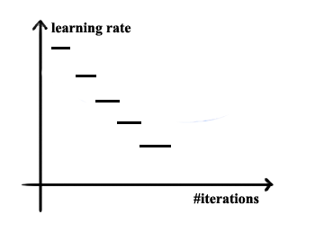 |
| manual decay | decrease learning rate manually day by day or hour by hour etc. |
- Batch Normalization
Batch Normalization at Train Time
Using batch normalization could speed up training.
The procedure is as follows.

The details of batch normalization in each layer $l$ is:
$\mu=\frac{1}{m}\sum Z^{(i)}$
$\delta^2=\frac{1}{m}\sum (Z^{(i)}-\mu)$
$Z^{(i)}_{normalized}=\alpha \frac{Z^{(i)}\mu}{\sqrt{\delta^2}+\epsilon} +\beta$
$\alpha$ and $\beta$ are learnable parameters here.
Batch Normalization at Test Time
At test time, we do not have the instances to compute $\mu$
and $\delta$, because probably we only have one test instance at each time.
In this situation, it is a good idea that estimating reasonable values of $\mu$ and $delta$ by using exponentially weighted average across mini-batches.
Paramters
- Learnable and Hyper Parameters
| Learnable Parameters |
|---|
| $W, b$ |
| Hyper Parameters |
|---|
| learning rate $\alpha$ |
| the number of iterations |
| the number of hidden layers $L$ |
| the number of hidden units of each layer |
| choice of activation function |
| parameters of Momentum |
| mini batch size |
| parameters of regularization |
- Parameters Initialization
(Note: Actually, the machine learning frameworks (e.g. tensorflow, chainer etc.) have already provided robust parameter initialization functions.)
Small Initial Values
For example, when we initialize the parameter $W$, we time a small value (i.e. 0.01) to ensure the initial parameters are small:
The reason for doing this is, if you are using sigmoid function and your initial parameters are large, the gradients would be very small.
More Hidden Units, Smaller Weights
Similarly, we will use pseudo-code to show how various initialization methods work. The idea is we prefer to assign smaller values to parameters to prevent the training phrase from vanishing or exploding gradients, if the number of hidden units is larger. The figure below may provide you some insights to understand the idea.
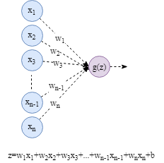
Based on the abovementioned idea, we could time the weights with a term related to the number of hidden units.
|
|
The equation of the multiplied term is $\sqrt{\frac{1}{n^{[l-1]}}}$. $n^{[l-1]}$ is the number of hidden units in the previous layer.
If you are using Relu activation function, using the term $\sqrt{\frac{2}{n^{[l-1]}}}$ could work better.
Xavier Initialization
If your activation function is $\tanh$, Xavier initialization ( $\sqrt{\frac{1}{n^{[l-1]}}}$ or $\sqrt{\frac{2}{n^{[l-1]} + n^{[l]}}}$) would be a good choice.
- Hyper Parameter Tuning
When tuning hyper parameters, it is necessary to try various possible values. If the computation resources are sufficient, the most simple way is training models with various parameter values parallel. However, most likely, the resources are very rare. In this case, we can just take care of only one model and try different values in different period.
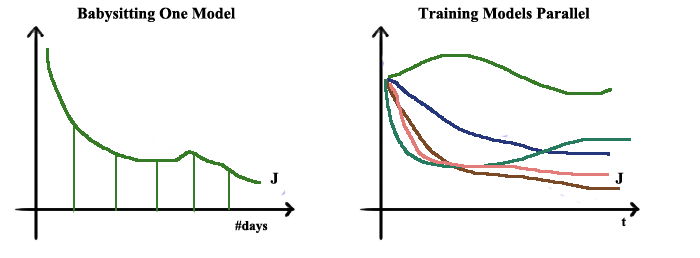
Apart from the abovementioned aspect, how to select the hyper parameter value wisely is also very important.
As you know, there are various hyper parameters in a neural network architecture: learning rate $\alpha$, Momentum and RMSprop parameters ($\beta_1$, $\beta_2$ and $\epsilon$), the number of layers, the number of units of each layer, learning rate decay parameters and mini-batch size.
The following priorities of hyper parameters were recommend by Andrew Ng:
| Priority | Hyper Parameter |
|---|---|
| 1 | learning rate $\alpha$ |
| 2 | $\beta_1$, $\beta_2$ and $\epsilon$ (parameters of momentum and RMSprop) |
| 2 | the number of hidden units |
| 2 | mini-batch size |
| 3 | the number of layers |
| 3 | the number of learning rate decay |
(usually, the default values of momentum and RMSprop are: $\beta_1=0.9$, $\beta_2=0.99$ and $\epsilon=10^{-8}$)
Uniform sample for hidden units and layers
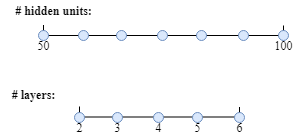
For example, if the range of layer numbers is 2-6, we can uniformly try to use 2, 3, 4, 5, 6 to train a model. Similarly, for the hidden units range 50-100, picking values in this scale is a good strategy.
Example:
Sample on log scale
You may have already realized that uniform sample is not usually a good idea for all kinds parameters.
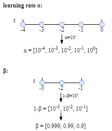
For instance, let us say an appropriate scale of learning rate $\alpha$ is $[0.0001,1]=[10^{-4},10^{0}]$. Obviously, picking values uniformly is unwise. A much better method is sampling on the log scale, $\alpha=10^r, r\in [-4,0]$ ($0.0001$, $0.001$, $0.01$, $0.1$ and $1$).
As for the parameter $\beta_1$ and $\beta_2$, we could use the similar strategy.
For example,
$1-\beta=10^r$
Therefore, $\beta=1-10^r$
$r\in [-3, -1]$
The table below could be helpful for you to understand the strategy better.
| $\beta$ | 0.9 | 0.99 | 0.999 |
| $1-\beta$ | 0.1 | 0.01 | 0.001 |
| $r$ | -1 | -2 | -3 |
Example:
Regularization
Regularization is a way to prevent overfitting problem in machine learning. An additional regularization term would be added to the loss function.
- L2 Regularization (weight decay)
$\min J(W,b)=\frac{1}{m}\sum_{i=1}^mL(\hat{y}^i,y^i)+\frac{\lambda}{2m}||W||_2^2$
In the new loss function, $\frac{\lambda}{2m}||W||_2^2$ is the regularization term and $\lambda$ is the regularization parameter (a hyper parameter). L2 regularization is also called weight decay.
For the logistic regression model, $W$ is a vector (i.e. the dimension of $W$ is the same as the feature vector), the regularization term would be:
$||W||_{2}^2=\sum_{j=1}^{dimension}W_{j}^2$.
For a neural network model which has multiple layers (e.g. $L$ layers), there are multiple parameter matrixes between layers. The shape of each matrix $W$ is $(n^{[l]}, n^{[l-1]})$. In the equation, $l$ is the $l^{th}$ layer and $n^{[l]}$ is the number of hidden units in layer $l$. Therefore, the L2 regularization term would be:
$\frac{\lambda}{2m}\sum_{l=1}^L||W^l||_2^2$
$||W^l||_{2}^2=\sum_{i=1}^{n^{[l-1]}}\sum_{j=1}^{n^{[l]}}(W_{ij}^l)^2$ (also called Frobenius norm).
- L1 Regularization
$\min J(W,b)=\frac{1}{m}\sum_{i=1}^mL(\hat{y}^i,y^i)+\frac{\lambda}{2m}||W^l||$
$||W^l||=\sum_{i=1}^{n^{[l-1]}}\sum_{j=1}^{n^{[l]}}W_{ij}^l$.
If we use L1 regularization, the parameters $W$ would be sparse.
- Dropout (inverted dropout)
To understand dropout intuitively, dropout regularization aims to make the supervised model more robust. In the training phrase, some output values of activation functions will be ignored. Therefore, when making predictions, the model will not rely on any one feature.
In dropout regularization, the hyper parameter “keep probability” describes the chance to active a hidden unit. Therefore, if a hidden layer has $n$ units and the probability is $p$, around $p \times n$ units will be activated and around $(1-p)\times n$ units will be shut off.
Example: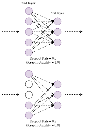
As shown above, 2 units of 2nd layer are dropped. Therefore, the value of linear combination of 3rd layer (i.e. $z^{[3]=}W^{[3]}a^{[2]}+b^{[3]}$) will decrease. In order not to reduce the expect value of $z$, we should adjust the value of $a^{[2]}$ by dividing the keep probability. That is: $a^{[2]} := \frac{a^{[2]}}{p}$
!Note: When making predictions at test time, there is NO NEED to use dropout regularization.
- Early Stopping
Using early stopping to prevent the model from overfitting.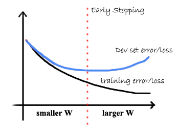
Models
- Logistic Regression
Given the feature vector of an instance $x$, the output of logistic regression model is $p(y=1|x)$. Therefore, the probability $p(y=0|x)=1-p(y=1|x)$. In a logistic regression, the learnable parameters are $W$ and $b$.
The x-axis is the value of $W^Tx+b$ and y-axis is $p(y=1|x)$. (The picture is download from wikipedia)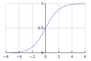
Loss function for one training instance $(x^i,y^i)$:
$\hat{y}^i$ is the prediction and $y^i$ is true answer.
Cost Function for the whole train dataset ($m$ is the number of examples in the training dataset):
Minimizing the cost function is actually maximizing the likelihood of data.
$LogLikelihood=\sum_{i=1}^{m}logP(y^i|x^i)=\sum_{i=1}^{m}log(\hat{y}^y(1-\hat{y})^{1-y})=-\sum_{i=1}^{m}L(\hat{y}^i,y^i)$
- Multi-Class Classification (Softmax Regression)
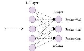
The softmax regression generalizes logistic regression (binary classification) to multiple classes (multi-class classification).
As shown in the figure above, it is a 3-class classification neural network. In the last layer, a softmax activation function is used. The outputs are the probabilities of each class.
The softmax activation is as follows.
1) $z^{[L]}=[z^{[L]}_0, z^{[L]}_1, z^{[L]}_2]$
2) $a^{[L]}=[\frac{e^{z^{[L]}_0}}{e^{z^{[L]}_0}+ e^{z^{[L]}_1}+e^{z^{[L]}_2}}, \frac{e^{z^{[L]}_1}}{e^{z^{[L]}_0}+e^{z^{[L]}_1}+ e^{z^{[L]}_2}}, \frac{e^{z^{[L]}_2}}{e^{z^{[L]}_0}+ e^{z^{[L]}_1}+e^{z^{[L]}_2}}]$
$=[p(class=0|x),p(class=1|x),p(class=2|x)]$
$=[y_0,y_1,y_2]$
Loss Function
$LossFunction=\frac{1}{m}\sum_{i=1}^{m}L(\hat{y^i},y^i)$
$L(\hat{y},y)=-\sum_j^{3}y_j^i\log\hat{y_j^i}$
$m$ is the number of train instances. $j$ is the j-th class.
- Transfer Learning
If we have a large amount of training data or our neural network is very big, it is time-consuming (e.g. a few days or weeks) for us to train such a model. Fortunately, there are some models released and available publicly. Usually, these models were trained on huge amount of data.
The idea of transfer learning is we can download these pre-trained models and adjust their models to our own problem as shown below.
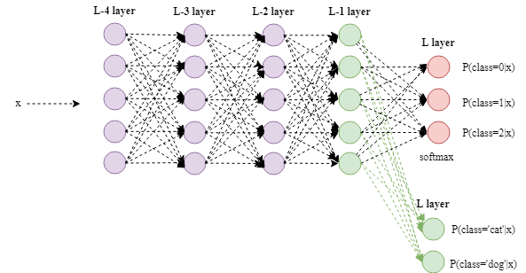
If we have a lot of data, we can re-train the whole neural network. On the other hand, if we have a small train set, we can retrain the last or last few layers (e.g. the last two layers).
In which situation we can use transfer learning?
Assume:
the pre-trained model is for task A and our own model is for task B.
- The two tasks should have the same input format
- For task A, we have a lot of training data. But for task B, the size of data size is much smaller
- The low level features learnt from task A could be helpful for training the model for task B.
- Multi-Task Learning
In a classification task, usually each instance only have one correct label as show below. The i-th instance only corresponds to the second class.
However, in a multitask learning, one instance may have multiple labels.
In the task, the loss function is:
$LossFunction=\frac{1}{m}\sum_{i=1}^{m}\sum_{j=1}^5 L(\hat{y^i_j},y^i_j)$
$L(\hat{y_j^i},y_j^i)=-y_j^i\log \hat{y_j}-(1-y_j^i)\log (1-y_j^i)$
$m$ is the number of train instances. $j$ is the j-th class.
Tips for multi-task learning:
- The multi-tasks learning model may share lower-level features
- we may can try a big enough neural network to work well on all the tasks
- In the train set, the amount of instances of each task is similar
- Convolutional Neural Network (CNN)
Filter/Kernel
For example, we have a $3*3$ filter (also called kernel) and the picture below describes how a filter/kernel works on a 2D input. The size of the input $x$ is $6*6$ and the size of the output when applying the filter/kernel is $4*4$.
The parameters (e.g. $w_1, w_2, …$) in filters/kernels are learnable.
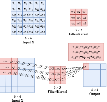
What is more, we can have multiple filters at the same time as shown below.
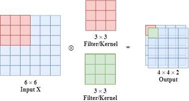
Similarly, if the input is a volume which has 3 dimensions, we can also have a 3D filter. In this filter, there are 27 learnable parameters.
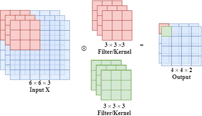
Usually, the width of filter is odd (e.g. $1*1$, $3*3$, $5*5$, …)
The idea of filter is if it is useful in one part of the input, probably it is also useful for another part of the input. Moreover, each output value of a convolutional layer output values only depends on a small number of inputs.
- Stride
Stride describes the step size of filter. It will affect the output size.
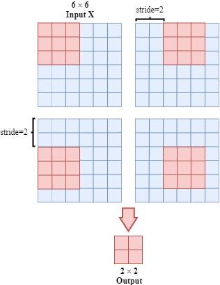
It should be noticed that some input elements are ignored. This problem can be solved by padding.
Back to Table of Contents
- Padding (valid and same convolutions)
As describe above, valid convolution is the convolution when we do not use padding.
Same convolution is we can use padding to extend the original input by filling zeros so that the output size is the same as the input size.
For example, the input size is $6*6$, and the filter is $3*3$. If we set stride=1 and padding=1, we can get the output with the same size as input.
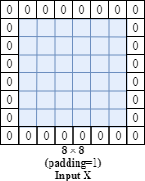
Generally, if the filter size is f*f, the input is n*n, stride=s, then the final output size is:
$(\lfloor \frac{n+2p-f}{s} \rfloor+1) \times (\lfloor \frac{n+2p-f}{s} \rfloor+1)$
- A Convolutional Layer
In fact, we also apply activation functions on a convolutional layer such as the Relu activation function.
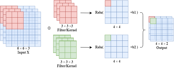
As for the number of parameters, for a filter, there are 27(parameters of filter) +1 (bias) =28 parameters totally.
- 1*1 Convolution
The problem of computational cost if we do not use 1X1 conv layer:
The number of parameter is reduced dramatically using 1X1 conv layer:
Back to Table of Contents
- Pooling Layer (Max and Average Pooling)
The pooling layer (e.g. max pooling or average pooling layer) could be considered as a special kind filter.
The max pooling layer returns the maximum number of the area which the filter currently covers. Similarly, the average pooling layers returns the average value of all the numbers in that area.
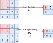
In the picture, $f$ is the filter width and $s$ is the value of stride.
Note: In a pooling layer, there is no learnable parameter.
- LeNet-5

(around 60k parameters in the model)
- AlexNet
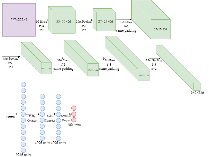
(around 60m parameters in the model; Relu activation function was used;)
- VGG-16

(around 138m parameters in the model; all the filters $f=3$, $s=1$ and using same padding; in the max pooling layer, $f=2$ and $s=2$)
Back to Table of Contents
- ResNet (More Advanced and Powerful)

$a^{[l+2]}=g(z^{[l+2]} + a^{[l]})$
- Inception Network
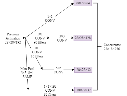
- Object Detection
- Classification with Localisation
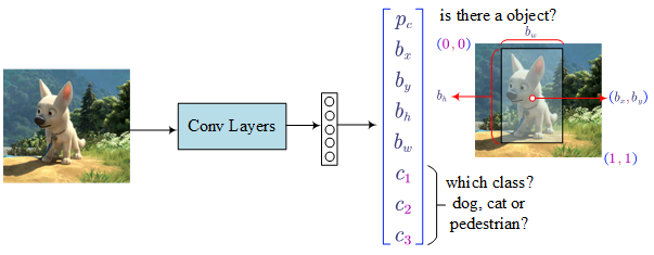
Loss Function:
Back to Table of Contents
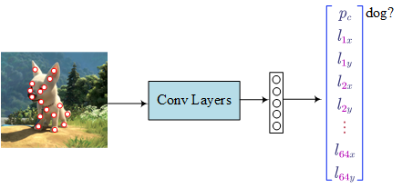
- Landmark Detection
- Sliding Windows Detection Algorithm
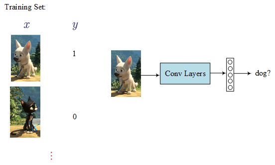
Firstly, using a training set to train a classifier. Then apply it to the target picture step by step:
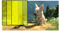
The problem is the computation cost (compute sequencently). In order to address this issue, we can use the convolutional implementation of sliding windows (i.e. turning the last fully connected layers into convolutional layers).
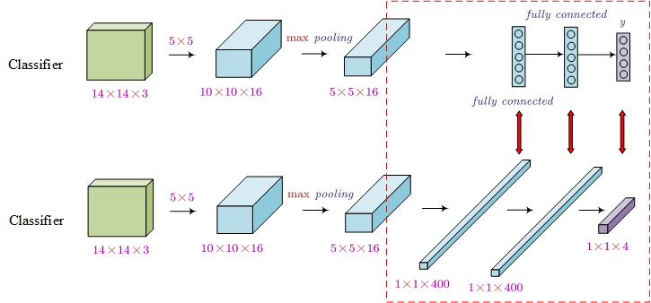
Using the convolutional implementation, we do not need to compute the results sequencently. Now we can compute the result once.

- Region Proposal (R-CNN, only run detection on a few windows)
In fact, in some pictures, there are only a few windows have the objects which we are interested in. In the region proposal (R-CNN) method, we only run the classifier on proposed regions.
R-CNN:
- use some algorithms to propose regions
- classify these proposed regions once at a times
- predict labels and the bounding boxes
Fast-R-CNN:
- use clustering methods to propose regions
- use convolution implementation of sliding windows to classify the proposed regions
- predict labels and bounding boxes
An other faster R-CNN is using convolutional network to propose regions.
- YOLO Algorithm
- Bounding Box Predictions (Basics of YOLO)
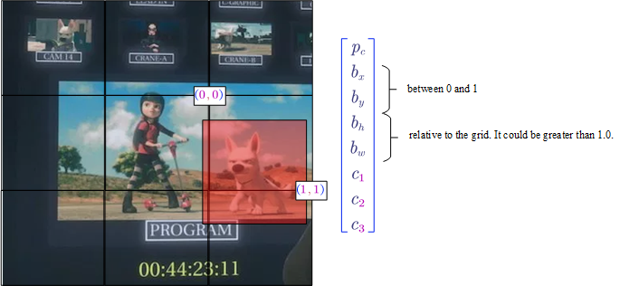
Each picture is divided into cells.
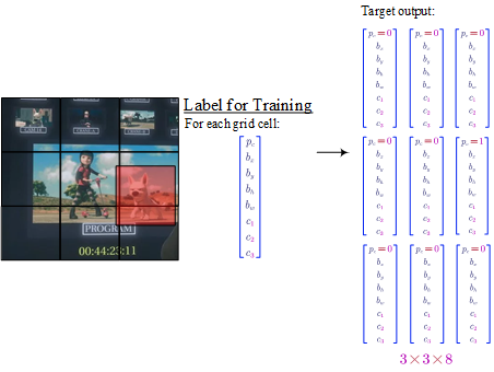
For each cell:
- $p_c$ denotes whether is there a object in the cell
- $b_x$ and $b_y$ is the mid point (between 0 and 1)
- $b_h$ and $b_w$ is the relative height and weight (the value could be greater than 1.0).
- $c_1$, $c_2$ and $c_3$ denote which class is the object belongs to.
- Intersection Over Union
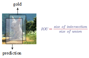
By convention, 0.5 is used very often to define as a threshold to judge as whether the predicted bounding box is correct or not. For example, if the intersection over union is greater than 0.5, we say the prediction is an correct answer.
$IOU$ can also be used as a way to measure how similar tow bounding boxes are to each other.
- Non-max Suppression
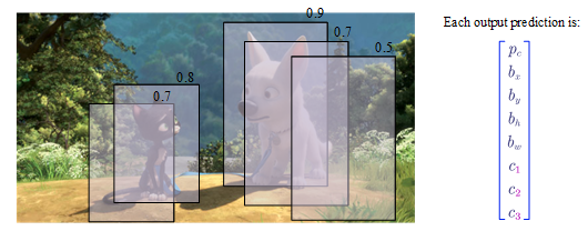
The algorithm may find multiple detections of the same objects. For example, in the above figure, it finds 2 bounding boxes for the cat and 3 boxes for the dog. The non-max suppression algorithm ensures each object only be detected once.
Procedure:
1) discard all boxes with $p_c \leq 0.6$
2) while there are any remaining boxes:
a. pick the box with the largest $p_c$ as a prediction outputs
b. discard any remaining box with $IOU \geq 0.5$ with the selected box in last step, and repeat from a.
- Anchor Boxes
The previous methods can only detect one object in one cell. But in some cases, there are more than one objects in a cell. To address this issue, we can per-define bounding boxes with different shapes.
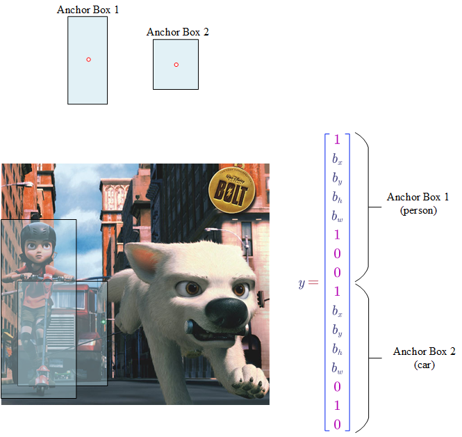
Therefore, each object in a training image is assigned to:
- a grid cell that contains the object’s mid point
- a anchor box for the grid cell with highest $IOU$
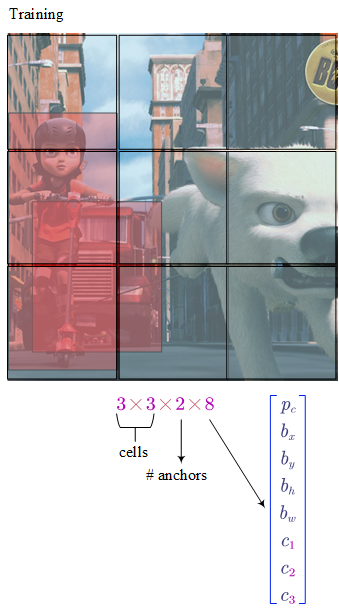
Making predictions:
- For each grid cell, we can get 2 (number of anchor boxes) predicted bounding boxes.
- Get rid of low probability Predictions
- For each class ($c_1$, $c_2$, $c_3$) use non-max suppression to generate final predictions.
- Face Verification
- One-Shot Learning (Learning a “similarity” function)
The one-shot learning in this situation is: learning from one example to recognise the person again.
The function $d(img1,img2)$ denotes the degree of difference between img1 and img2.

- Siamese Network (Learning difference/similar degree)
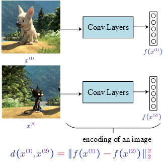
If we believe the encoding function $f(x)$ is a good representation of a picture, we can define the distance as shown in the bottom of the above figure.
Learning:
Learnable parameters: parameters of the neural network defining an encoding $f(x)$
Learn these parameters so that:
- if $x^{(i)}$ and $x^{(j)}$ are the same person, $||f(x^{(i)}) - f(x^{(j)})||^2$ is smaller
- if $x^{(i)}$ and $x^{(j)}$ are the different people, $||f(x^{(i)}) - f(x^{(j)})||^2$ is large
- Triplet Loss (See three pictures at one time)
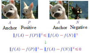
The three pictures are:
- Anchor Picture
- Positive Picture: another picture of the same person in the anchor picture
- Negative Picture: another picture of not the same person in the anchor picture.
But there would be a problem just learning the above loss function. This loss function may lead to learning $f(A)=f(P)=f(N)$.
To prevent from this problem, we can add a term smaller than zero, i.e., $||f(A)-f(P)||^2-||f(A)-f(N)||^2 \leq 0-\alpha$.
To reorganise it:

To summarise the loss function:

Choose the triples of A, P, N:
During training, if A, P, N are chosen randomly, it is easy to satisfied $d(A,P) + \alpha \leq d(A,N)$. The learning algorithm (i.e. gradient descent will not do anything).
We should choose triples that are hard to train on.

When using hard triples to train, the gradient descent procedure has to do some works to try to push these quantities further away from quantities.
- Face Recognition/Verification and Binary Classification
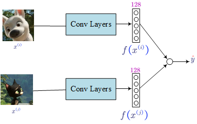
we can learn a sigmoid binary classification function:

We can also use other variations such as chi square similarity:
- Neural Style Transfer
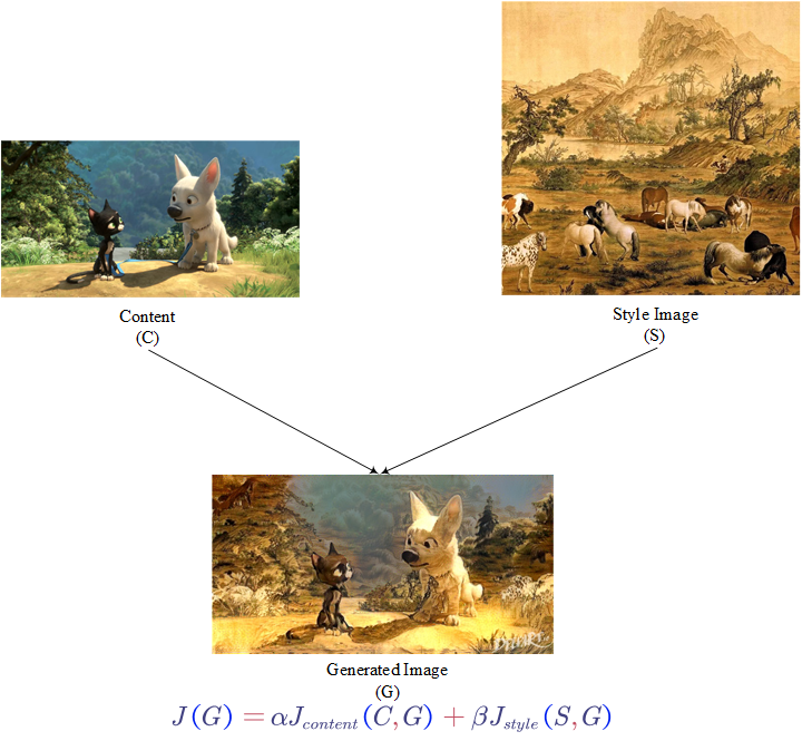
The content image is from the movie Bolt.
The style image is a part of One Hundred Stallions, one of the most famous Chinese ancient paintings.
The generated image is supported by https://deepart.io.
The loss function $J$ contains two parts: $J_{content}$ and $J_{style}$. To find the generated image $G$:
- Randomly initialise image $G$
- Use gradient descent to minimise $J(G)$
Content Cost Function, $J_{content}$:
The content cost function ensures that the content of the original image is not lost.
1) use a hidden layer (not too deep and also not too shallow), $l$, to compute the content cost. (we can use the layer $l$ from a pre-trained CONV neural network)

2)
3)
Style Cost Function, $J_{style}$:
1) say we are using layer $l’s$ activation to measure style.
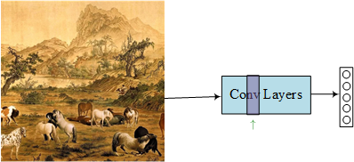
2) define the style of an image as correlation between activations across channels
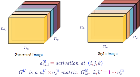
The elements in matrix $G$ reflects how correlated are the activations across different channels (e.g. whether or not high level texture components tend to occur or not occur together).
For style image:
For generated image:
Style Function:
You may can also consider combine the style loss of different layers.

- 1D and 3D Convolution Generalisations
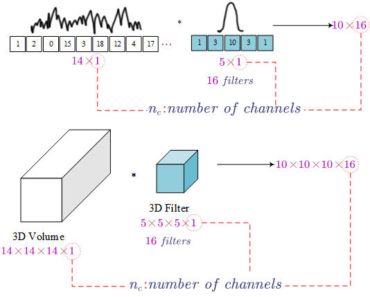
Sequence Models
- Recurrent Neural Network Model
Forward: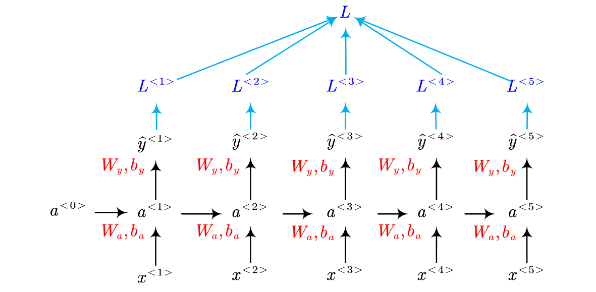
In this figure, the red parameter are learnable variables, $W$ and $b$. In the end of each step, the loss of this step is computed.
Finally, all the loss of each step are summed up as the total loss, $L$, for the whole sequence.
Here is the formula for each step: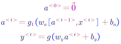
The total loss: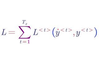
Backpropagation Through Time: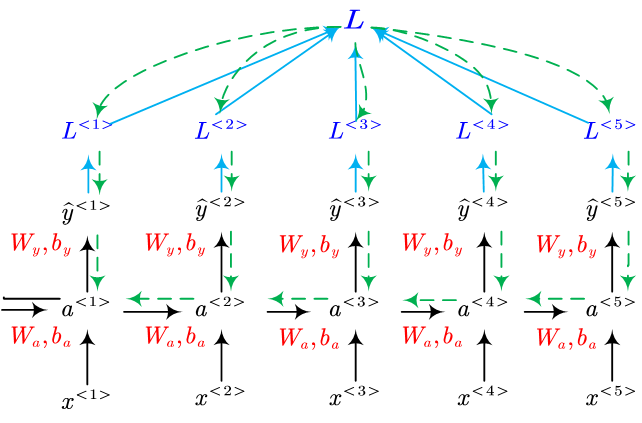
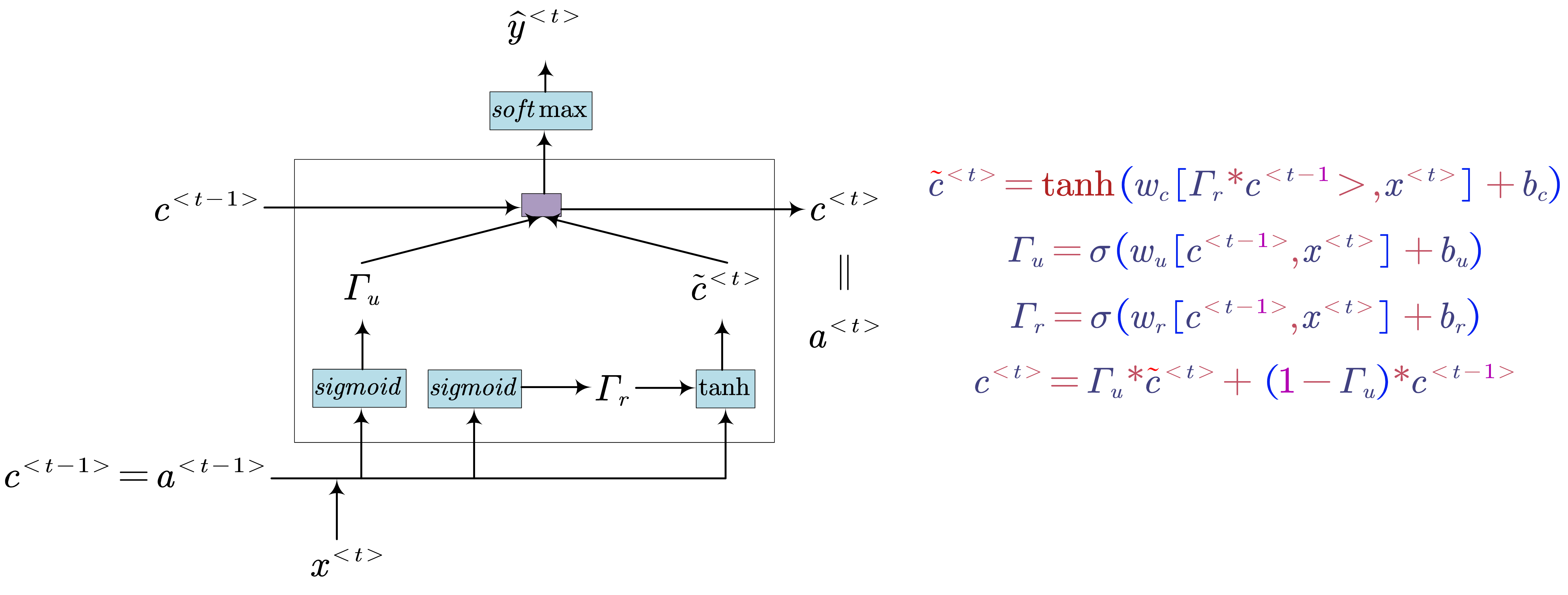
- Gated Recurrent Unit (GRU)
- GRU (Simplified)
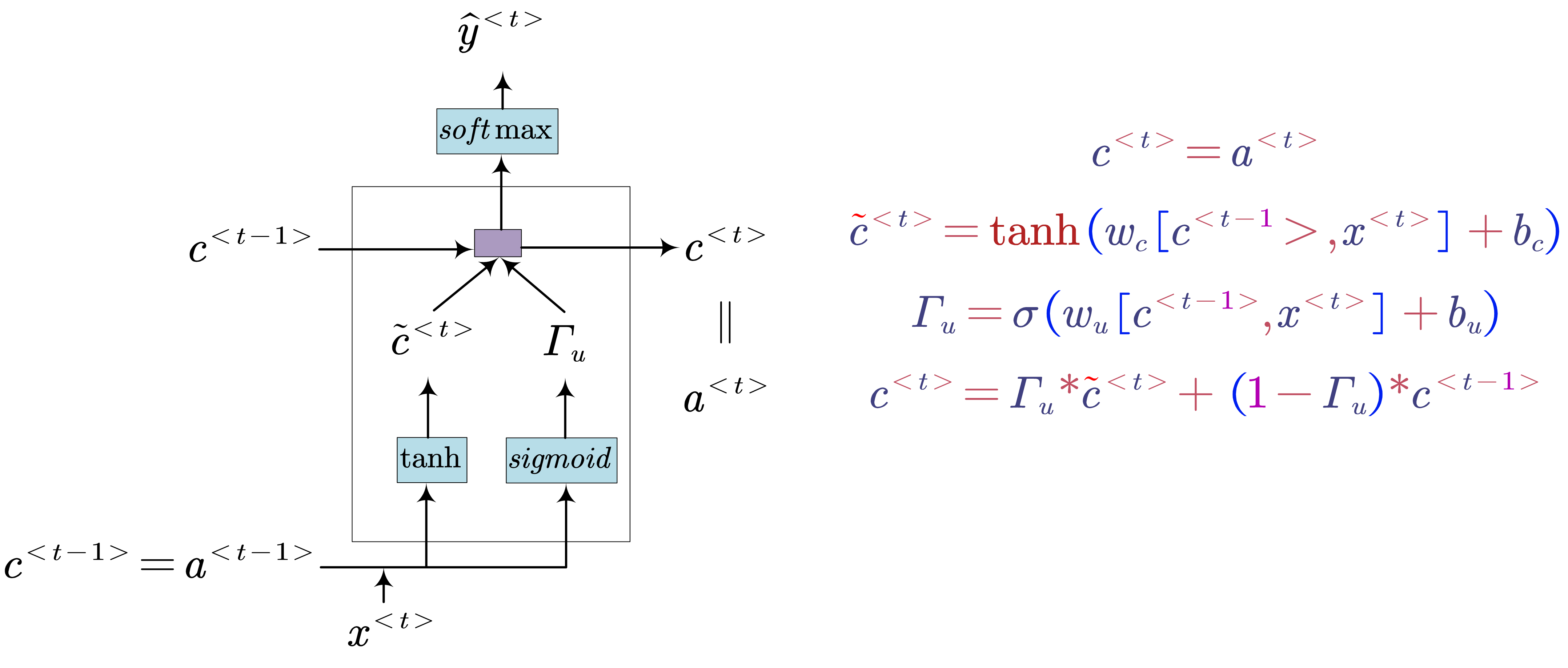
- GRU (Full)
- Long Short Term Memory (LSTM)
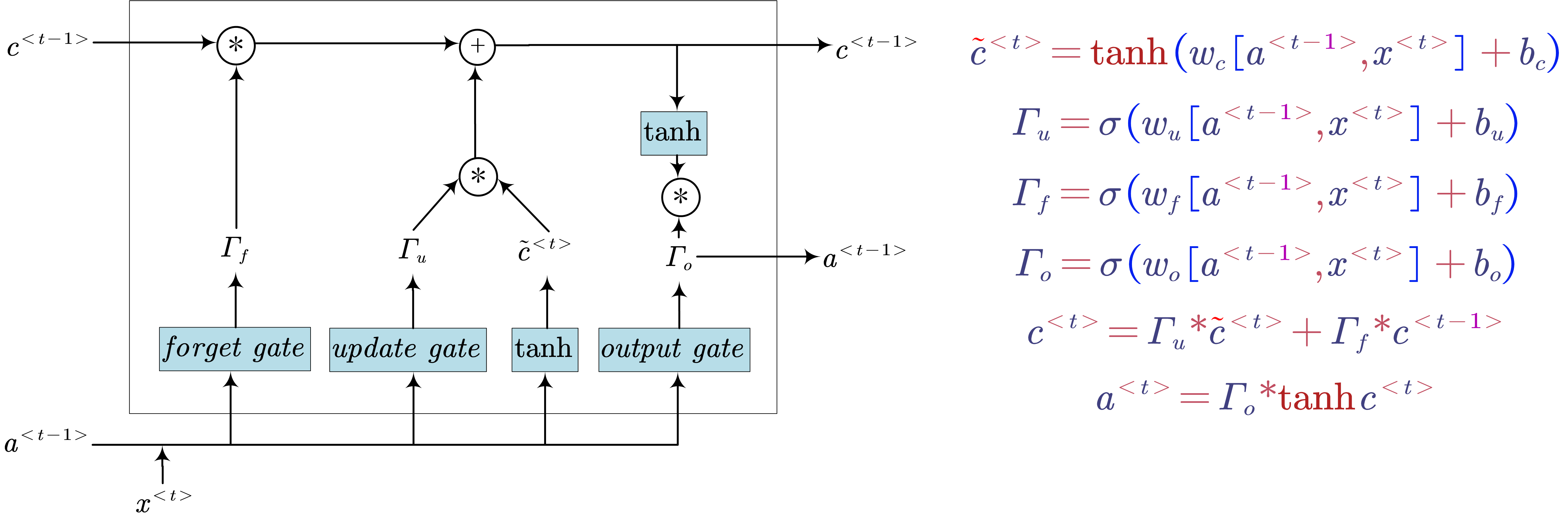
- $u$: update gate
- $f$: forget gate
- $o$: output gate
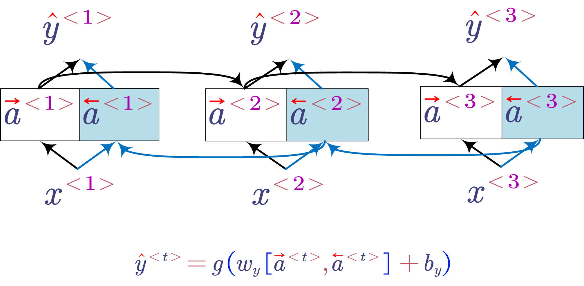
- Bidirectional RNN
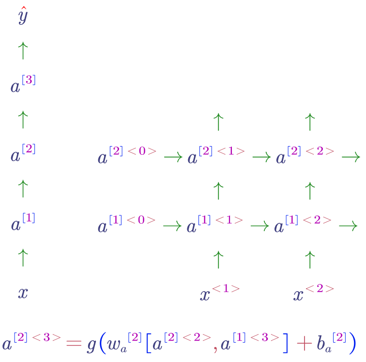
- Deep RNN Example
- Word Embedding
- One-Hot
- Embedding Matrix ($E$)
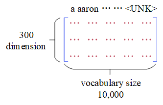
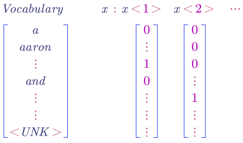
The $UNK$ is a special work which represents unknown words. All the unseen words will be casted to $UNK$.
The matrix is denoted by $E$. If we want to get the word embedding for a word, we can use the word’s one-hot vector as follows: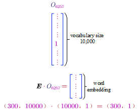
In general, it can be formulised as:
Back to Table of Contents
- Learning Word Embedding
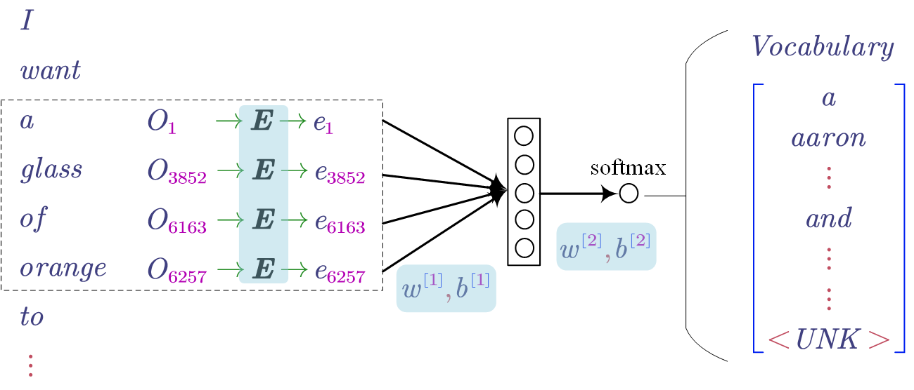
In the model, the embedding matrix (i.e. $E$) is learnable as the same as the other parameters (i.e. $w$ and $b$). All the learnable parameters are highlighted by blue.
The general idea of the model is predicting the target word given its context. In the above figure, the context is the last 4 words (i.e. a, glass, of, orange) and the target word is “to”.
In addition, there are different ways to define the context of the target word such as:
- last $n$ words
- $n$ words left and right the target word
- nearby one word (idea of Skip-gram)
- …
- Word2Vec & Skip-gram
Sentence: I want a glass of orange juice to go along with my cereal.
In this word embedding learning model, the context is a word randomly picked from the sentence. The target is a word randomly picked up with a window of the context word.
For example:
let us say the context word is ‘orange’, we may get the following training examples.

Model: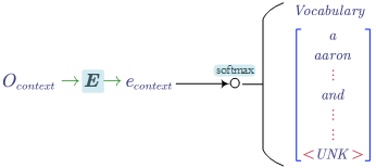
The softmax function is defined as:

$\theta_t$ is the parameter associate with the output and $e_c$ is the current embedding for the context word.
The problem of using the softmax function is the computation cost of denominator is too much as we may have a very large vocabulary. In order to reduce the computation, negative sampling is decent solution.
- Negative Sampling
Sentence: I want a glass of orange juice to go along with my cereal.
Given a pair of words (i.e. context word an another word), and a label (i.e. whether the second word is the target word). As shown in the below figure, the (orange juice 1) is a positive example as the word juice is the real target word of orange. Because all the other words are randomly selected from dictionary, these words are considered as wrong target words. So these pairs are negative examples (it is ok if the real target word is selected as a negative example by chance).
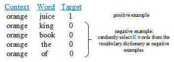
As for the number of negative words for each context word, if the dataset is small, $k=5-20$ and if the dataset is a very large one, $k=2-5$.
Model:
We only train $K+1$ logistic regression models of the softmax function. Thus the computation is much lower and cheaper.
How to choose negative examples?: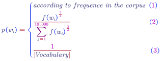
$f(w_i)$ is the word frequency.
if we use the first sample distribution, we may always select words like the, of, and etc. But if we use the third distribution, the selected words would be non-representative. Therefore, the second distribution could be considered as a better one for sampling. This distribution is at somewhere between the first one and the third one.
- GloVe Vector
Notation: $X_{ij} = $ number of times word $i$ appears in the context of word $j$
Model:
$X_{ij}$ measures how related are those two words and how often these two words occurs together. $f(X_{ij})$ is a weight term. It gives high frequency pairs not too high weights and also gives less common pairs not too little weights.
If we check the math of $\theta$ and $e$, actually they play the same role. Therefore, the final word embedding of a word is:

- Deep Contextualized Word Representations (ELMo, Embeddings from Language Models)
Pre-train bidirectional language model
Forward language model: Given a sequence of $N$ tokens, $(t_1,t_2,…,t_N)$, a forward language model compute the probability of the sequence by modelling the probability of $t_k$ given the history, i.e.,

Backward language model: similarly,
Bidirectional language model: it combines both a forward and backward language model. Jointly maximize the likelihood of the forward and backward directions:
LSTMs are used to model the forward and backward language models.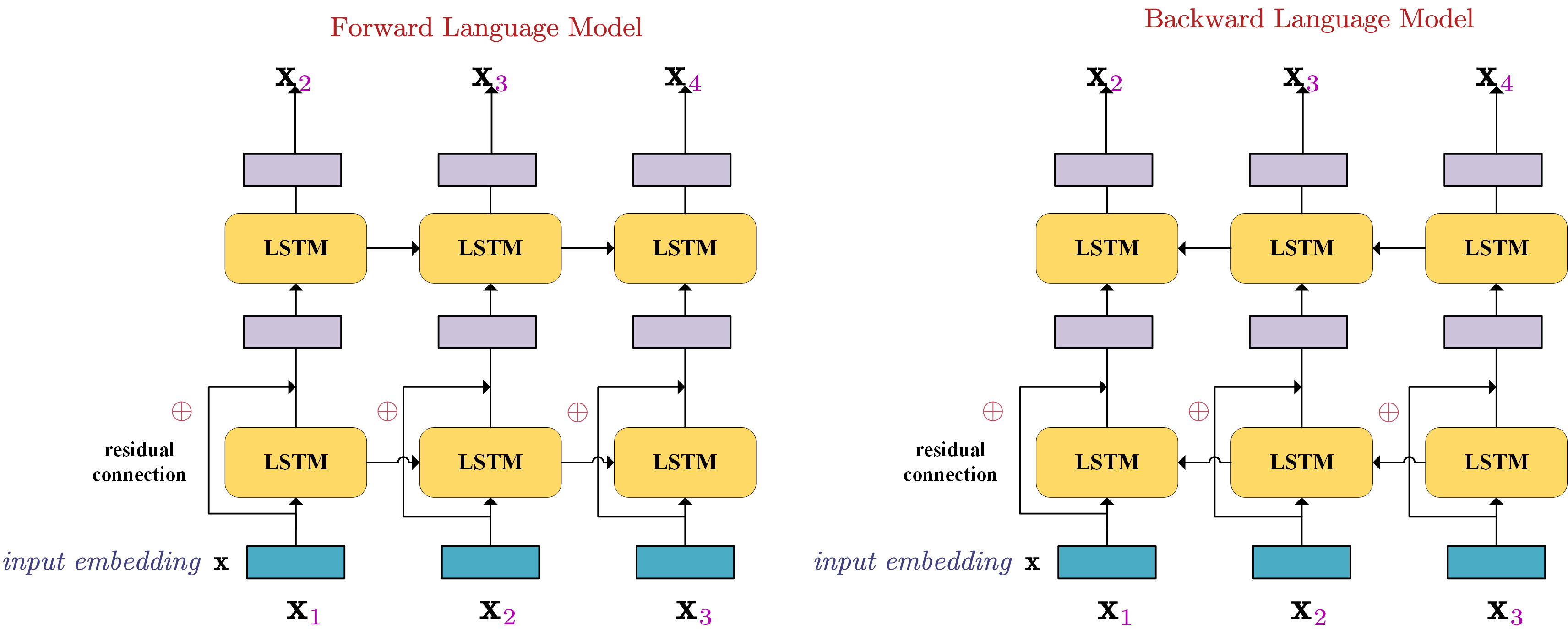
In terms of the input embeddings, we can just initialise these embeddings or use a pre-trained embedding. For ELMo, it is a bit more complicated by using character embeddings and convolutional layer as shown below.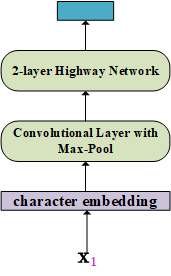
After the language model is trained, we can get the ELMo embedding of a word in a sentence: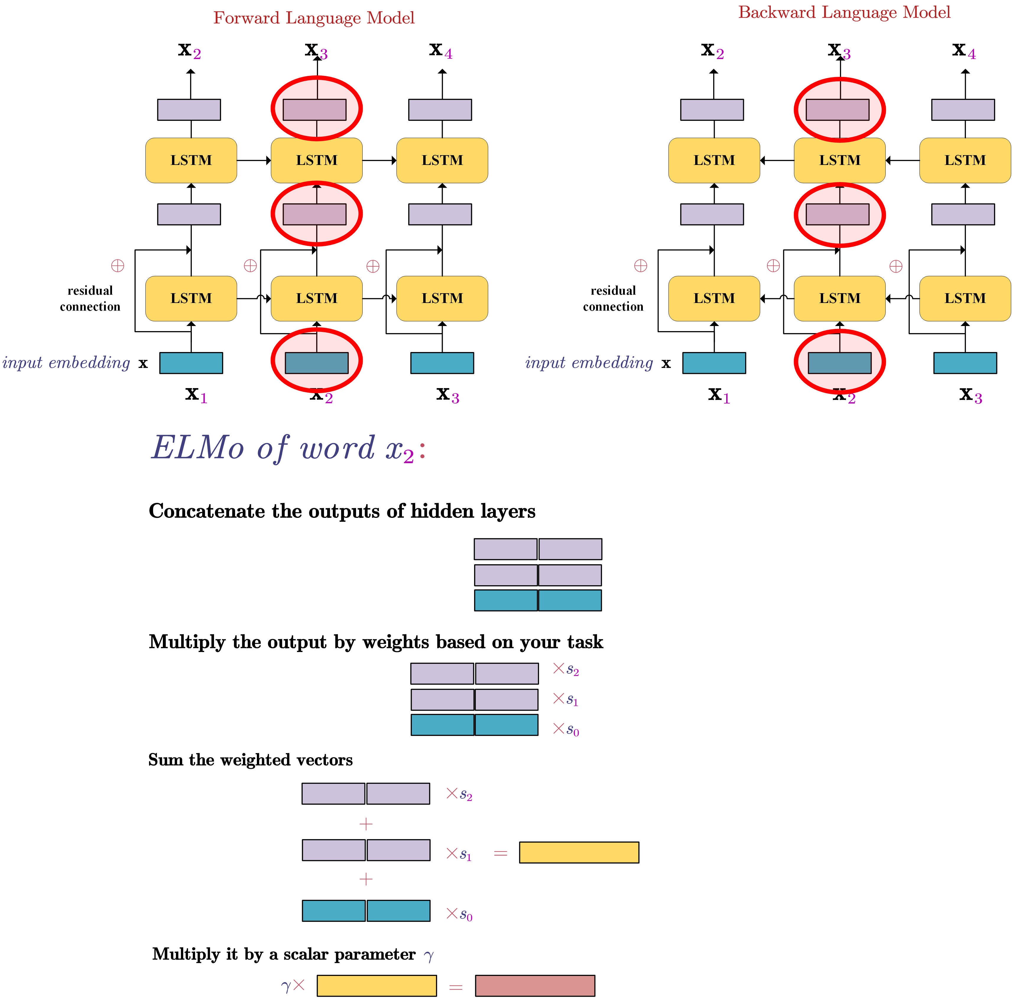
In the ELMo, $s$ are softmax-normalized weights and $\gamma$ is the scalar parameter allows the task model to scale the entire ELMo vector. These parameters can be learned during tarining of the task-specific model.
Reference:
[1] https://www.slideshare.net/shuntaroy/a-review-of-deep-contextualized-word-representations-peters-2018
[2] http://jalammar.github.io/illustrated-bert/
[3] https://www.mihaileric.com/posts/deep-contextualized-word-representations-elmo/
- Sequence to Sequence Model Example: Translation
The task is translate a sequence to another sequence. The two sequences may have different length.


- Pick the most likely sentence (Beam Search)
- Beam Search
Using sequence to sequence models is popular in machine translation. As shown in the figure, the translation is generated token by token. One of the problems is how to pick up the most likely whole sentence? The greedy search does not work (i.e. pick the best word at each step). Beam Search is a much better solution to this situation.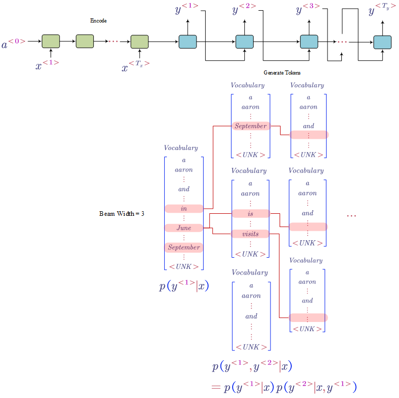
Let us say the beam search width is 3. Therefore, at each step, we only keep the top 3 best prediction sequences.
For example (as shown in the above picture),
- at step 1, we keep in, June, September
- at step 2, we keep the sequences: (in, September), (June is), (June visits)
- …
As for the beam search width, if we have a large width ,we can get better result, but it would make the model slower. One the other hand, if the width is smaller, the model would be faster but it may hurt its performance. The beam search width is a hyper parameter and the best value maybe domain dependent.
- Length Normalisation
The learning of the translation model is to maximise:
In the log space that is:
The problem of the above objective function is that the score in log space is always negative, therefore using this function will make the model prefers a very short sentence. We do not want the translation is too short actually.
We can add a length normalisation term at the beginning:
Back to Table of Contents
- Error Analysis in Beam Search (heuristic search algorithm)
When tuning the parameters of the model, we need to decide the priority of them (i.e. which is more to blame, the RNN or the beam search part). (Usually increasing beam search width will not hurt the performance).
Example
Pick a sentence from the dev set and check our model:
Sentence: Jane visite l’Afrique en septembre.
Translation from Human: Jane visits Africa in September. ($y^*$)
Output of the Algorithm (our model): Jane visited Africa last September. ($\hat{y}$)
To figure out which one is more to blame, we need to compute and compare $p(y^*|x)$ and $p(\hat{y}|x)$ according to the RNN neural network.
if $p(y^*) > p(\hat{y}|x)$:
$y^{*}$ obtains a higher probability, we can conclude that the beam search is at fault.
if $p(y^*) \leq p(\hat{y}|x)$:
The RNN predicted $p(y^*) \leq p(\hat{y}|x)$, but actually $y^*$ is a better translation than $\hat{y}$ as it is from a real human. Therefore, the RNN model should be at fault.
By repeating the above error analysis process on multiple instances in the dev set, we can get the following table: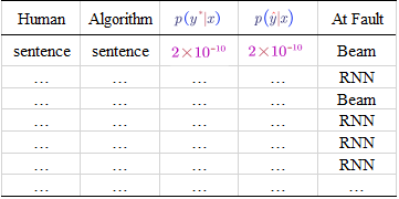
Based on the table, we can figure out what faction of errors are due to beam search/RNN.
If most of the error are due to the beam search, just try to increase the beam search width. Otherwise, we may try to make the RNN more deeper/add regularisation/get more training data/try different architectures.
Back to Table of Contents
- Bleu Score
If there are multiple great answers/references for one sentence, we can use Bleu Score to measure our model’s accuracy.
Example (Bleu Score on bigrams):
French: Le chat est sur le tapis.
Reference1: The cat is on the mat.
Reference2: There is a cat on the mat.
The output of our model: The cat the cat on the cat.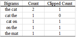
The Count is the number of current bigrams appears in the output. The Clipped Count is the maximum number of times that the bigram appears in either reference 1 or reference 2.
Then the Bleu Score on bigrams can be computed as:

The above equation can be used to compute unigram, bigram or any-gram Bleu scores.
- Combined Bleu
The combined Bleu score combines the scores on different grams. $p_n$ denotes the Bleu Score on n-grams only. If we have $P_1$, $P_2$, $P_3$ and $P_4$, we can combined as following:

The brevity penalty penalises short translation. (we do not want translation very short as short translations will lead high precisions.
- Attention Model
One problem of RNN (e.g. lstm) is it is hard for it to memorise a super long sentence. The model translation quality would decrease as the length of original sentence increases.
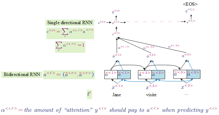
There are different ways to compute the attention. One way is:
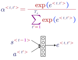
In this method, we use a small neural network to map the previous and current information to an attention weight.
It has already been proven that attention models work very well such as normalisation.

- Transformer (Attention Is All You Need)
Architecture: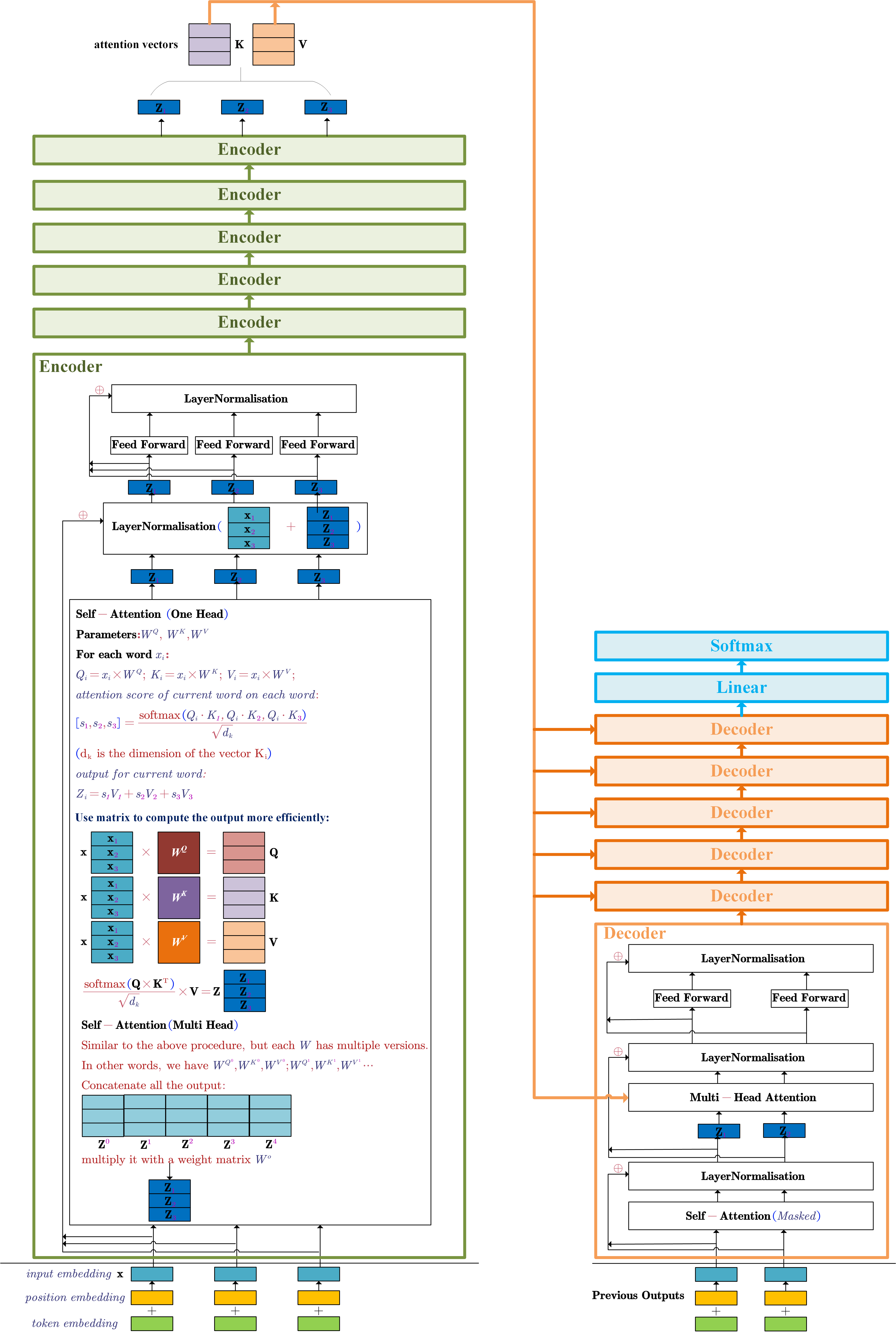
Details:
Input Embeddings
The input embeddings of the model are the summation of the word embedding and its position encoding for each word. For example, for the input sentence $\mathbf{x}=[\mathbf{x_1},\mathbf{x_2},\mathbf{x_3}]$. $\mathbf{x}$ are the word embeddings (could be a pre-trained embedding) for each word in the sentence. The input embedding should be $[\mathbf{x_1} + \mathbf{t_1},\mathbf{x_2} + \mathbf{t_2},\mathbf{x_3} + \mathbf{t_3}]$.
$[\mathbf{t_1,t_2,t_3}]$ are the position encodings of each word. There are many ways to encode the word position. In the paper, the used encoding method is:
$t_{position,2i}=sin(\frac{pos}{10000^{\frac{2i}{dmodel}}})$
$t_{position,2i+1}=cos(\frac{pos}{10000^{\frac{2i}{dmodel}}})$
$position$ is the position of the word in the sentence. $i$ is the element position of the position encoding. $dmodel$ is the output dimension size of the encoder in the model.
Decoder
- the output of the top encoder is transformed into attention vectors $K$ and $V$. These are used in the multi-head attention sublayer (also named encoder-decoder attention). The attention vectors can help the decoder focus on useful places of the input sentence.
- the masked self-attention is only allowed to attend to earlier positions of the output sentence. Therefore, the future positions are masked by setting them to -inf before the softmax step.
- the “multi-head attention” layer is similar to the self-attention layer in encoder, except:
- it takes the $K$ and $V$ from the output of the top encoder
- it creates the $Q$ from the layer below it
Reference: https://jalammar.github.io/illustrated-transformer/
- Bidirectional Encoder Representations from Transformers (BERT)
BERT is built by stacking Transformer Encoders.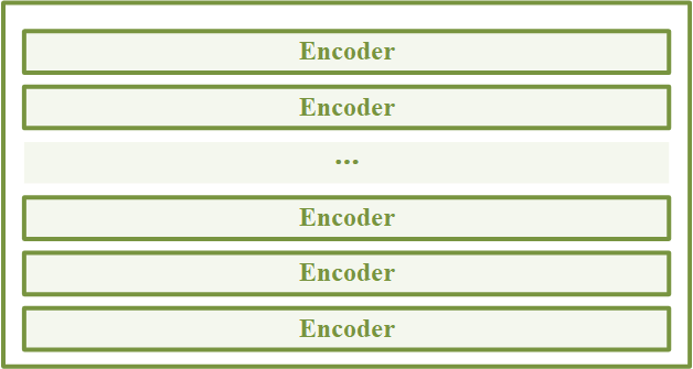
Pre-train the model on large unlabelled text (predict the masked word)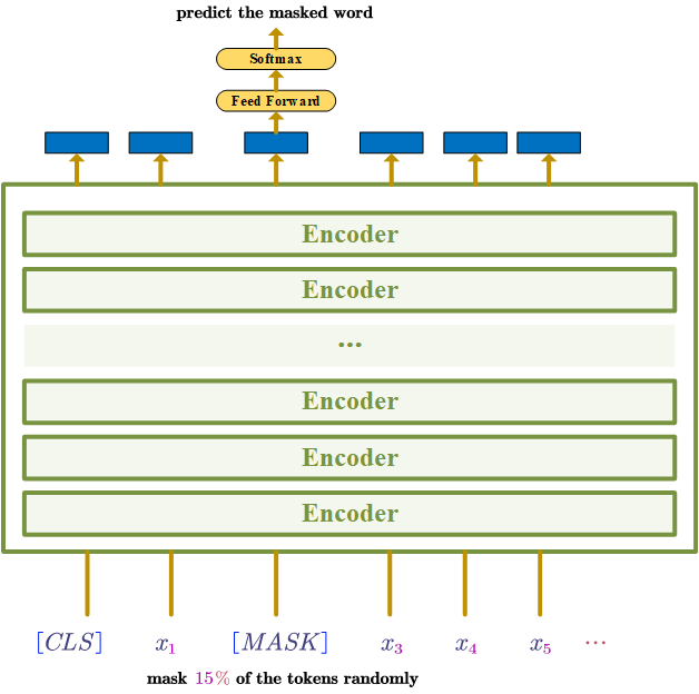
“The masked language model randomly masks some of the tokens from the input, and the objective is to predict the original vocabulary id of the masked word based only on its context.” [2]
Use supervised train to fine-tune the model on a specific task, e.g. classification task, NER etc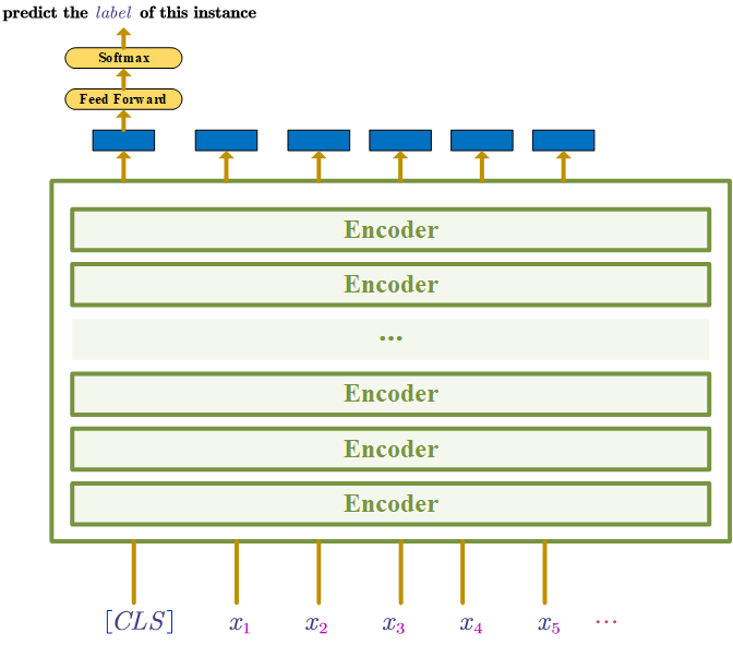
The figure below from the BERT paper shows how to use the model to different tasks.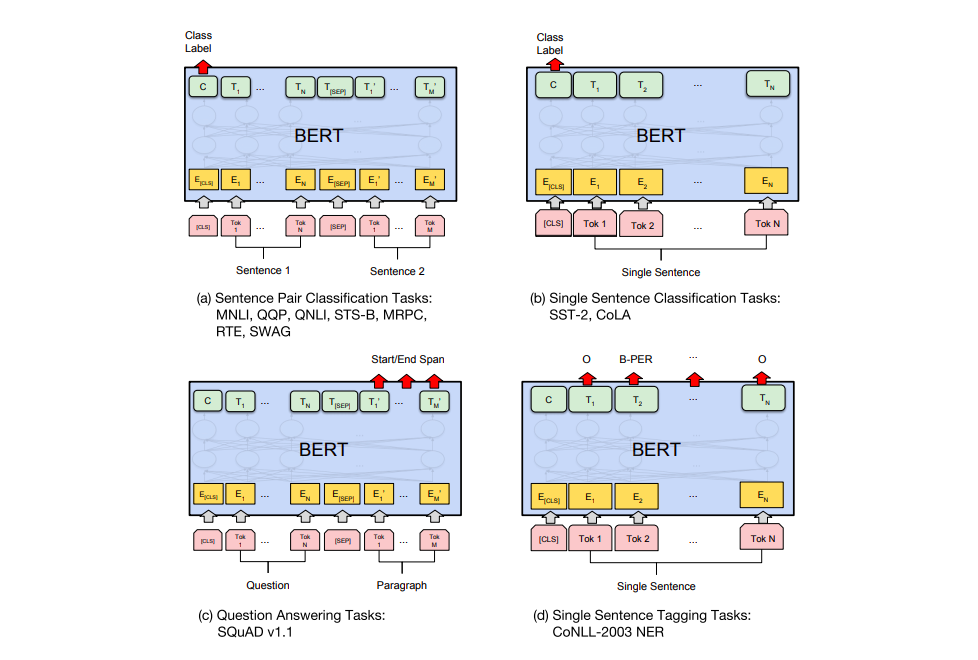
If the specific-task is not a classfication task, the [CLS] can just be ignored.
Reference:
[1] http://jalammar.github.io/illustrated-bert/
[2] Devlin, J., Chang, M.W., Lee, K. and Toutanova, K., 2018. Bert: Pre-training of deep bidirectional transformers for language understanding. arXiv preprint arXiv:1810.04805.
Practical Tips
- Train/Dev/Test Dataset
- Usually, we use 70% of a dataset as training data and 30% as test set; or 60%(train)/20%(dev)/20%(test). But if we have a big dataset, we can use most of the instances as training data (e.g. 1,000,000, 98%) and make the sizes of dev and test set equally (e.g. 10,000 (1%) for dev and 10,000 (1%) for test set). Because our dataset is big, 10,000 examples in dev and test set are more than enough.
- Make sure the dev and test set come from the same distribution
Another situation we maybe in is:
1) we want to build a system for a specific domain, but we only have a few labelled dataset in that domain (e.g. 10,000)
2) we can get a much larger dataset (e.g. 200,000 instances) from similar tasks.
In this case, how to build our train, dev and test set?
The easiest way is just combine the two datasets and shuffle it. Then we can divide the combined datasets into three parts (train, dev and test set). BUT it is not a good idea. Because our goal is to build a system for our own specific domain. There is no point that adding some instances which is not from our own domain into the dev/test dataset to evaluate our system.
The reasonable method is:
1) all the instances (e.g. 200,000) which are available more easily are added into the training set
2) Pick some instances from the specific domain datasets and add them into the training set
3) Divide the remain instances of our own domain into dev and test set

- Over/UnderFitting, Bias/Variance, Comparing to Human-Level Performance, Solutions
Over/UnderFitting, Bias/Variance
For a classification task, the human classification error is supposed to be around 0%. The analysis of various possible performances of the supervised model on the both training and dev set is as shown below.
| Human-Level Error | 0.9% | 0.9% | 0.9% | 0.9% |
| Training Set Error | 1% | 15% | 15% | 0.5% |
| Test Set Error | 11% | 16% | 30% | 1% |
| Comments | overfitting | underfitting | underfitting | good |
| high variance | high bias | high bias and variance | low bias and variance |
Solutions: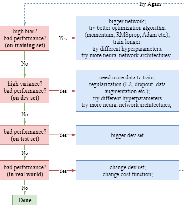
Comparing to Human-Level Performance
You may have noticed that, in the table above, the human-level error was set 0.9%, what if the human-level performances are different but the train/dev errors are the same?
| Human-Level Error | 1% | 7.5% |
| Training Set Error | 8% | 8% |
| Test Set Error | 10% | 10% |
| Comments | high bias | high variance |
Although the model errors are the same, in the left case where the human error is 1%, we have the problem of high bias and have the high variance problem in the right case.
As for the performance of model, sometimes it could work better than that of human. But so long as the model performance is worse than human’s, we can:
1) get more labelled data from humans
2) gain insights from manual error analysis
3) gain insights from bias/variance analysis
- Mismatched Data Distribution
When we are building a system for our own specific domain, we only have a few labelled instances (e.g. 10,000) for our own problem. But it is easy for us to collect a lot of instances (e.g. 200,000) from another similar domain. Moreover, the large amount of easily available instances could be helpful to train a good model. The dataset may look like this:

But in this case, the data distribution of training set is different with dev/test set. This may cause side effects - data mismatch problem.
In order to check whether we have the data mismatch problem, we should randomly pick up a subset of training set as a validation set named train-dev dataset. This set has the same distribution of training set, but will not be used for training.

| Human-Level Error | 0% | 0% | 0% | 0% |
| Train Error | 1% | 1% | 10% | 10% |
| Train-Dev Error | 9% | 1.5% | 11% | 11% |
| Dev Error | 10% | 10% | 12% | 20% |
| Problem | high variance | data mismatch | high bias | high bias + data mismatch |
To summarize:

Addressing the Mismatch Data Distribution Problem
Firstly, making a manually error analysis to try to understand what is the difference between our training set and dev/test set.
Secondly, according to the analysis result, we can try to make the training instances more similar to the dev/test instances. We can also try to collect more training data similar to the data distribution of dev/test set.
- Input Normalization
We have a train set including $m$ examples. $X^{(i)}$ represents the $i^{th}$ exmaple. The inputs normalization is as follows.
$X:=\frac{X-\mu}{\sigma^2}$,
$\mu=\frac{1}{m}\sum_{i=1}^mX^{(i)}$,
$\sigma^2=\frac{1}{m}\sum_{i=1}^m(X^{(i)})^2$
!Note: MUST use the same $\mu$ and $\sigma^2$ of training data to normalize the test dataset.
Using input normalization could make training faster.
Suppose the inputs are two dimensional, $X = [X_1, X_2]$. The ranges are [1-1000] and [1-10] of $X_1$ and $X_2$ respectively. The loss function may look like this (left):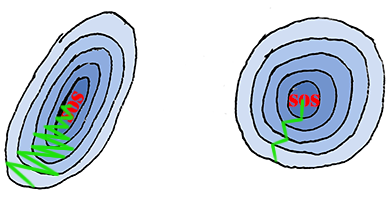
- Use a Single Number Model Evaluation Metric
If we not only care about the performance of model (e.g. accuracy, F-score etc.), but also the running time, we can design a single number evaluation metric to evaluate our model.
For example, we can combine the performance metric and running time such as $metric=accuracy-0.5*RunningTime$.
Alternatively, we can also specify the maximal running time we can accept:
$max: accuracy$
$subject: RunningTime <= 100ms$
- Error Analysis (Prioritize Next Steps)
Doing error analysis is very helpful to prioritize next steps for improving the model performance.
Carrying Out Error Analysis
For example, in order to find out why the model mislabelled some instances, we can get around 100 mislabelled examples from the dev set and make an error analysis (manually check them one by one).
| Image | Dog | Big Cat | Blurry | Comments |
|---|---|---|---|---|
| 1 | $\surd$ | |||
| 2 | $\surd$ | |||
| 3 | $\surd$ | $\surd$ | ||
| … | … | … | … | … |
| percentage | 8% | 43% | 61% |
By manually checking these mislabelled instances one by one, we can estimate where are the errors from. For example, in the abovementioned table, we found 61% images are blurry, therefore in the next step, we can mainly focus to improve the performance in blurry images recognition.
Cleaning Up Incorrectly Labelled Data
Sometimes, our dataset is noisy. In other words, there are some incorrect labels in the dataset. Similarly, we can pick up around 100 instances from dev/test set and manually check them one by one.
For example, currently the model error on dev/test set is 10%. Then we manually check the randomly picked 100 instances from the dev/test set.
| Image | Incorrect Label |
|---|---|
| 1 | |
| 2 | $\surd$ |
| 3 | |
| 4 | |
| 5 | $\surd$ |
| … | … |
| percentage | 6% |
Let’s say, finally we found 6% instances were labelled incorrectly. Based on it, we can guess around $10\%*6\%=0.6\%$ errors due incorrect labels and $9.4\%$ errors due other reasons.
Therefore, if we focus on correcting labels maybe not a good idea in the next step.
